Playing Around

Cloudy Forecast: How Predictable is Communication Latency in the Cloud?

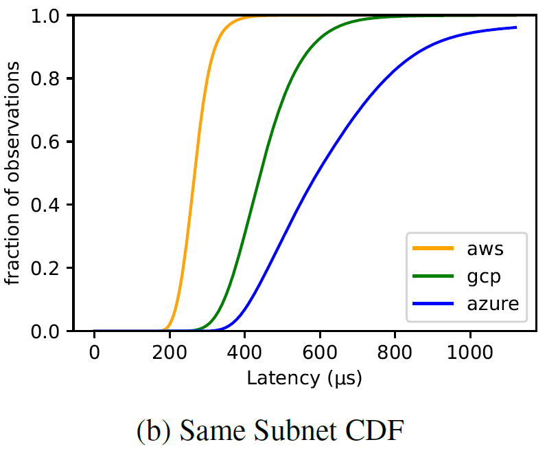
Many, if not all, practical distributed systems rely on partial synchrony in one way or another, be it a failure detection, a lease mechanism, or some optimization that takes advantage of synchrony to avoid doing a bunch of extra work. These partial synchrony approaches need to know some crucial parameters about their world to estimate how much synchrony to expect. A misjudgment of such synchrony guarantees may have significant negative consequences. While most practical systems plan for periods of lost partial synchrony and remain safe, they may still pay the performance or availability cost. For example, a failure detector configured for a very short timeout may cause false positives and trigger unnecessary and avoidable misconfigurations, which may increase latency or even make systems unavailable for the duration of reconfiguration. Similarly, a system that uses tight timing assumptions to remain on an optimized path may experience performance degradation when such synchrony expectations do not hold. One example of the latter case is EPaxos Revisited and their TOQ optimization that uses tight assumptions about communication delays in the cluster to avoid conflicts and stay on the “fast path.”

More recently, the partial synchrony window has been shrinking in systems, with many algorithms expecting timeouts or tolerances of under ten milliseconds. Moreover, some literature proposes schemes that work best with sub-millisecond timing tolerances. However, how realistic are these tight timing tolerances?

Systems use timing assumptions to manage the communication synchrony expectations. For example, failure detectors check whether the expected heartbeat message has arrived in time. Systems relying on synchrony for “fast path” use timing assumptions, explicitly or implicitly, to judge the existence of messages—if nothing has arrived in some time window, then a system may expect that nothing has been sent in the first place. For instance, algorithms like Rabia or EPaxos Revisited TOQ rely on this assumption implicitly, as the protocol expects some message to arrive at all participating nodes at nearly the same time for optimal performance. A node that has not received the message in time will be in a mismatched state and potentially cause a delay when the algorithm needs to check/enforce safety.

Anyway, to decide whether the tight timing tolerances required by some protocols are realistic, we need to look at what communication latency underlying infrastructure can provide. This communication latency is end-to-end latency between two processes running in different nodes in some infrastructure, such as the cloud. Many factors impact this end-to-end, process-to-process communication latency. Starting from the obvious, the network between nodes plays a major role, but the communication goes through other layers as well, such as virtualization, OS kernel, and even the application/system process itself.

Last semester, in my seminar on the reliability of distributed systems, some students and I did a little experiment measuring this end-to-end latency in various public clouds to see what timing assumptions are realistic. We prepared a report and even tried to publish it twice, but it seems the reviewers do not care about our trivially collected observations (more on this in the “Rant” section at the end).

See, measuring end-to-end latency is not hard. Ping utility does that. So, we wrote a Cloud Latency Tester (CLT), essentially a bigger ping utility that works over TCP sockets, sends messages of configured size at a configured rate across many deployed instances, and finally records the round trip time between all pairs of nodes. CLT works in rounds — each node sends a ping message to all peers and expects the peers to respond with a corresponding pong message carrying the same payload. Each node records the round-trip latency observed for each peer in each ping round. The rounds also allow for the extrapolation of additional information, such as quorum latency.

We then deployed CLT in the big three (AWS, Azure, and GCP) on some of their more popular VMs and let it run. For the deployment, we wanted to test some meaningful scenarios, such as latency within the same AZ of a region, across three AZs of a region, and across several cloud regions. The figure illustrates the deployment strategy we followed for all cloud providers. For nodes inside the AZ, we also tried to see if separating them into different subnets made any difference (it did not); hence, some nodes in the same AZ appear in different subnets. And for VM choice, we settled on supposedly popular but small VM instances — all VMs had 2 vCPUs and 8 GB of RAM and similar enough network bandwidth. Finally, we let CLT cook for 6 hours between 2 and 8 p.m. on the weekday at a rate of 100 rounds per second at each node with 1024 bytes of payload.

Below, I summarize our observations and lessons learned. Note that our goal was not to compare the cloud vendors; instead, we wanted to know what engineers can expect from latency between processes — how small or large it is and how predictable it appears. Let’s start with a high-level summary overview:

The box-plot summary for round-trip latency over a 6-hour interval, starting at 2 pm EST on a weekday. The box denotes the IQR, with the middle line designating the median, while the whiskers represent the 5th and 95th percentiles. The green triangle shows the average latency. Note that we are not comparing clouds, so the subfigures have different scales to better show data for each cloud provider. Figure (d) shows latency summary for in-house cluster.

This summary figure illustrates a few things. For one, talking to oneself is not very fast. While it is faster than talking to a process in remote VMs, even that is not always the case. Second, we can expect some decent variability in communication latency. Just a pick at Azure figure shows 95th percentile latency gets closed to 1.5 ms, almost 2× the average latency! Finally, as expected, cross-AZ communication overall is slower in all clouds and tends to have higher variance.

Now, let’s zoom in on each cloud provider. The figure below shows 30-second latency averages for each provider:

Round-trip latency averaged over 30-second widnows between nodes in the same subnet of the same AZ in East1 region over a 6-hour interval, starting at 2 pm EST on the weekday.

An obvious feature of AWS data is two big latency spikes. While looking at the raw data, the culprit seemed to be a few smaller spikes happening within a few seconds of each other. The highest such spike clocked at 832.83 ms or 2,900× the average latency. It occurred at one node in one communication round for all peers except oneself. Since the loopback communication worked without a problem, we think that the problem was external to the VM. Azure data is very puzzling. Aside from showing frequent spikes above 1 ms for many 30-second windows, the data also suggests the existence of some cyclical pattern with a roughly 20-minute cadence. GCP data seemed the most boring among the three. Finally, we also include a similar measurement on equipment in our lab; to our delight, aside from the few big spikes, AWS data looks similar to what we get in our hardware.

The figure below takes a look at the same latency data, but presents it as a latency histogram and latency CDF:

Same AZ round-trip latency distribution over a 6-hour interval.

With this figure, we see a lot of interesting stuff. For one, Azure has the longest tail towards high latency that fades very slowly. AWS and GCP seem more predictable in this regard, with observation looking more Normal. The Azure’s tail was so bad, that we had to cut it out from the CDF figure for space reasons — the 99th percentile exceeded 2.5 ms!

The next figure shows latency between individual pairs of nodes in the same subnet of the same AZ:

Same Subnet/AZ round-trip latency over a 6-hour interval for individual pairs of nodes.

Of the peculiar observations here are the changes in latency that happen over time. For instance, there is a noticeable increase in latency on AWS after 15,000 seconds of run time. On GCP, a similar increase exists but only on some nodes. The cyclical patterns on Azure are more visible in this figure.

Finally, let’s look at some data for talking across AZs:

Cross-AZ round-trip latency distribution over a 6-hour interval.

Here we can easily see multi-modal latency distributions — it appears that, at least in AWS and Azure, the latency/distance between AZs is not uniform, which results in different pairs of nodes having different latency. It is worth noting that similar behavior can be observed even within the same AZ — depending on the placement of VMs inside the AZ, some pairs may be quicker than others. I will not put the figure for this, but it is available in the report.

Finally, I want to talk briefly about quorums. Quorums are powerful communication primitives used in many data-intensive protocols. Quourms allow the masking of failed nodes, but also mask the slowest nodes, so looking at quorum latency makes a lot of sense for such systems:

Box plots for round-trip latency over a 6-hour interval with quorums. NQ stands for no-quorum distribution, representing a simple node-to-node communication. Q2/3 is a majority quorum of two nodes out of three for each communication round. Q3/3 is an all-quorum, requiring a response from all nodes in each round.

Here, as expected, a quorum of 2 out of 3 nodes appears a bit faster than individual messages or waiting for all peers in the cluster (i.e., a quorum of all nodes captures the worst-case latency). What is missing from the box plots is very extreme tail latency, and this is where quorums excel — at 99.999th percentile, the 2-out-of-3 quorum latency is better than individual message latency by up to 577X in our measurements.

I think I will stop with figures here; the report has more stuff, including the discussion of cross-region latency. Our goal was to see what communication latency one can expect in the cloud, and I think we got some pretty interesting data. The bottom line is that I do not think the general purpose cloud is ready yet for sub-millisecond timing assumptions that a lot of academic literature is pursuing now. There are a few other implications for my academic friends — testing/benchmarking systems in the cloud can be tricky — your latency can noticeably change over time. Also, unless you are careful with node placement (and picking leaders in leader-based systems), that placement can impact latency observations.

Rant Time

This is an observation study that, in my opinion, shows some useful/interesting data for system builders/engineers. This study treats the cloud as a black box, exactly as it appears for cloud users, and measures the end-to-end latency as observed by processes running on different nodes in the cloud. It does not try to break down the individual factors contributing to the latency. While these factors may be very useful for cloud providers and their engineering teams to troubleshoot and optimize their infrastructure, for cloud users, it is irrelevant whether the high latency is caused by the cloud network, virtualization technology, or bad VM scheduling. What matters for cloud users is the latency their apps/systems see, as these latencies also drive the safe timing assumptions engineers can take. I believe this point was one of the reasons the JSys reviewers rejected the report — the reviewers wanted to see the network latency and got the end-to-end one. However, the report clearly states that in the very first figure that shows what exactly we measure.

Of course, this observation study is far from perfect, and several factors could have influenced our observations, such as hidden failures in the cloud providers, using only relatively small VMs, and running only for a few hours. The reviewers, of course, are eager to point out these “problems,” again, despite the report clearly stating these deficiencies. However, running things for longer will not solve the latency variations we already observed in 6 hours. If anything, it will show more stuff and more patterns, such as daily latency fluctuations. Longer runs do not invalidate the plethora of observations we made with just a handful of shorter runs. Similarly, trying with bigger VMs will give more valuable and complete data. Maybe (and likely) bigger VM instances will be more stable. However, smaller instances are still more numerous in the cloud, making our observations valid for many users.

Anyway, the report is now on arxiv, and I am done with this little project.

PigPaxos: continue devouring communication bottlenecks in distributed consensus.

pigpaxos

This is a short follow-up to Murat’s PigPaxos post. I strongly recommend reading it first as it provides full context for what is to follow. And yes, it also includes the explanation of what pigs have to do with Paxos.

Short Recap of PigPaxos.

In our recent SIGMOD paper we looked at the bottleneck of consensus-based replication protocols. One of the more obvious observations was that in protocols relying on a single “strong” leader, that leader is overwhelmed with managing all the communication. The goal of PigPaxos is to give the leader a bit more breathing room to do the job of leader, and not talking as much. To that order, we replaced the direct communication pattern between leader and followers with a two-hop pattern in which a leader talks to a small subset of randomly picked relay nodes, and the relays in turn communicate with the rest of the cluster. PigPaxos also uses relays to aggregate the replies together before returning to the leader. On each communication step, PigPaxos uses a new set of randomly picked relay nodes to both spread the load evenly among the followers and to tolerate failures.

pigpaxos_communication

By randomly rotating the relays and enforcing timeouts and including some other optimization on how many nodes to wait at each relay node, we can provide adequate performance even in the event of node crashes or network partitions. The fault tolerance limit of PigPaoxs is similar to Paxos, and up to a minority of nodes may fail with the system still making some (limited if implemented naively) progress.

Some More Results

In the original PigPaxos post, we have not talked about scaling to super large clusters. Well, I still do not have that data available, but following the footsteps of our SIGMOD work, we have developed a performance model that, hopefully, is accurate enough to show some expected performance on the bigger scale.

pigpaxos_model
Performance Model of PigPaxos on for a cluster of 25 and 99 nodes and 3 relay groups.

Network uniformity is not a requirement for PigPaxos. In fact it is perfectly ok to have some links slower than the others. However, some arrangement of relay groups may be required to get the best performance when links between nodes have different speed or capacity.  The most pronounced real-world example of this non-uniformity is the wide area networks. When we deployed real, not-simulated PigPaxos in such geo-distributed environment, it no longer had the disadvantage of slower latency, as the latency became dominated by much slower geo-links. We took advantage of natural division between fast and slow links, and made all nodes in every region to be part of the same relay group. Another advantage of this setup is the amount of cross-region traffic flowing, as data moves to each region only once regardless of how many replicas are there.

pigpaxos_wan

On the fault tolerance front, relay nodes definitely introduce more ways for the protocol to stumble. Crash of a relay node makes the entire relay group unavailable for that communication attempt. Crash of a non-relay node causes timeout which may add to the operation latency. The core principle behind PigPaxos’ fault tolerance is to repeat failed communication in the new configuration of relay nodes. Eventually, the configuration will be favorable enough to make progress, given that the majority of nodes are up. However, this process can be slow when many nodes are crashed, so some orthogonal optimization can help. For example, it is worth remembering nodes temporarily down and not use these nodes for relays or otherwise expect them to reply on time. Another approach is to reduce the wait quorum of the relay group to tolerate strugglers, or even use overlapping groups for communication redundancy. However, even with all these ad-hoc optimizations turned off, PigPaxos can still mask failures originating in the minority of relay groups without much impact on performance. For example, in the experiment below we have one relay group experiencing a failure on every operation for 10 seconds without much detriment to overall performance.

pigpaxos_crash

Why Scaling to This Many Nodes?

One of the most important questions about PigPaxos is “why?” Why do you need this many nodes in Paxos? Well, the answer is not simple and consists of multiple parts:

  •         Because we can!
  •         Because now we can tolerate more nodes crashing
  •         Because now we can make services like ZooKeeper or even databases to scale for reads just by adding more nodes. ZooKeeper reads are from a single node. And so are many databases that provide some relaxed consistency guarantees.
  •         Because it allows bigger apps with more parties that require consensus. And it is done by a single protocol.


Keep The Data Where You Use It

As trivial as it sounds, but keeping the data close to where it is consumed can drastically improve the performance of the large globe-spanning cloud applications, such as social networks, ecommerce and IoT. These applications rely on some database systems to make sure that all the data can be accessed quickly. The de facto method of keeping the data close to the users is full replication. Many fully replicated systems, however, still have a single region responsible for orchestrating the writes, making the data available locally only for reads and not the updates.

Moreover, full replication becomes rather challenging when strong consistency is desired, since the cost of synchronizing all database replicas on the global scale is large. Many strongly consistent datastores resort to partial replication across a handful of nearby regions to keep the replication latency low. This creates situations when some clients close to the regions in which data is replicated may experience much better access latency than someone reaching out from the other side of the globe.

Data and consumer are collocated.
No access penalty when data and consumer are in the same region

Data and consumer are in different regions
Access penalty (289 ms in this case) when data and consumer are in different regions

Despite the obvious benefits of adapting to locality changes, many databases offer only static partitioning. Of course, some data stores have the migration capability, but still often lack the mechanisms to determine where the data must be moved. Quite a few orthogonal solutions provide capabilities to collocate related data close together or use days or weeks’ worth of logs to compute better data placement offline. Meanwhile, Facebook’s aggressive data migration helps them reduce the access latency by 50% and save on both storage and networking.

We (@AlekseyCharapko, @AAilijiang and @MuratDemirbas) investigated the criteria for quick, live data migration in response to changes on access locality. We posit that effective data-migration policies should:

  • Minimize access latency,
  • Preserve load balancing with regards to data storage and processing capacity
  • Preserve collocation of related data, and
  • Minimize the number of data migrations.

Policies

We developed four simple migration policies aimed at optimizing the data placement. Our policies operate at an arbitrary data-granularity, be it an individual key-value pairs, micro-shards, or the partitions. For simplicity, I say that policies work on objects that represent some data of an arbitrary granularity.

The main point we address with the policies is minimizing access locality, with each policy using a different heuristic to make a data-placement decision. Once the policy finds the most optimal location for an object, it checks the load balancing constraints to adjust the data migration decision as required.

Our simplest policy, the n-consecutive accesses policy, uses a threshold of consecutive accesses to the object to make the placement decision. Although simple, this policy works well for workloads with strong locality in a single region. Majority accesses policy keeps track of some request statistics and uses it to find the region with the most accesses to an object over some time interval. It then migrates the data over to that region.

The exponential moving average (EMA) policy takes a different approach and computes the average region for all requests to the object. The average region is computed as an exponential moving average favoring the most recent requests. This policy can potentially find better placement for objects that have more than one high-access region. However, it requires the regions to have numerical IDs arranged in the order of region’s proximity to each other. This policy falters for deployments with complicated geography and may require multiple migrations to move data to the best location. Another disadvantage of EMA is that it takes longer to settle and requires many data migrations. Unlike other policies that can move the data directly to the desired region, EMA can only migrate objects to one of the neighboring regions, making adjustment such as going from region (1) to (3) include a temporary migration to region (2).

Exponential moving average topology; regions have left and right neighbors

Finally, the center-of-gravity (CoG) policy calculates the optimal object placement by taking into account the distribution of all requests to an object and the distances between the datacenters. CoG policy calculates the region closest to the central location for any access locality workloads. CoG can collect the request statistics similar to the majority accesses policy and make a placement decision only after some time has elapsed since last decision. Alternatively, it can use a continuous metric to assign each region a score corresponding to its weight in the workload, adjust the score and recompute the best object placement with every request.

CoG
Computing CoG Weights (L-scores). Region with lowest score is most central to the current workload’s access distribution. Japan is the object’s owner here, despite Australia having more requests overall. L_jp = 0.4 * 128 + 0.15 * 165 + 0.13 * 318 + 0.08 * 165 = 130.49

Some Evaluation

I’ve simulated protocols under different access locality scenarios and calculated the latency of inter-region access and the number of object movements each policy makes. In the simulations, I used 3000 distinct objects, initially assigned to a random region in the cluster of 15 regions. I used the AWS inter-region latencies to specify the distances between simulated regions.  To my surprise, even the most basic policies showed good improvement over static random placement of data.

In the first experiment, the objects were accessed according to a normal distribution. Each object has a ID assigned to it, and some Normal distribution dictates the probability of the drawing the ID each region. All regions have distributions with the same variance, but different means, making each region predominantly accessing some of the objects, and having some group of objects being more-or-less shared across the regions with adjacent IDs.

Locality Workload. 3000 Objects, 15 regions. Probability of object access is controlled by N(200z,100), where z is region ID in range [0, 15)
In this experiment, both CoG and majority accesses policy showed the best results in terms of latency and the number of object movements. This is because the workload almost always favors a single region, and in rarer cases shares the object between two regions. This makes majority heuristic that only considers one region work well. Similarly, 3-consecutive accesses policy shows good latency, but it generates a lot of jitter constantly moving shared objects between neighboring regions.

When the workload is no longer predominantly single region dominant for every key, single-region heuristic policies perform worse. For instance, equally sharing an object between utmost 3 regions out of 15 causes majority and 3-consecutive accesses policies to lock in to one of the sharing regions instead of optimizing the latency for all sharing regions. CoG policy can place the data in a region optimal for all 3 regions (and not even necessarily in one of the sharing regions) and optimize the latency better than a single-region heuristic, topology unaware policies. EMA policy is at a big disadvantage here, since it relies on ID assignments to dictate the proximity of regions. However, the complex geography of AWS datacenters makes a good ID assignment nearly impossible, causing EMA to sometimes overshoot the best region and settle in less optimal one.

Access is shared equally with up to 3 random regions.

Access locality may fluctuate on a regular basis, and the policy needs to be able to adopt to such changes and adjust the system to keep the latencies low. In this experiment I gradually adjust the normal distribution used in the earlier experiment to make a gradual workload switch. In the figure below, the system ran for enough time to make all objects switch the access locality to the neighboring region. However, the policies adopt well to the change, keeping low latency despite the moving workload. EMA is one notable exception again, as it first gets better latency and the gradually degrades until reaching a steady state (In a separate experiment I observe EMA stabilizing over at around 59 ms of latency)

Changing access locality

Previous experiments did not consider the effect of load balancing. However, a good data-migration policy should refrain from migrating data to overloaded regions. In the next experiment I applied load-balancing filter to the CoG policy to make the migration procedure first compute the best region for the object, check if that region has the capacity, and if no capacity is available, move the data to the next best region with enough processing/storage capacity. Here I used 5 regions and 1000 objects, and limited each region to storing at most 25% of all data. I ran a heavily skewed workload with 80% of all requests coming from a single region. Under these conditions the CoG policy achieves very low average latency. However, as evidenced by the disbalance graph, all objects migrate over to a single region.  If load balancing is enabled, no region becomes overloaded, but latency improvement becomes more modest.

Balancing
Balancing enabled. Latency on the left, disbalance measured as the difference in object ownership between most and least loaded region


Concluding Remarks

Having data close to the consumers can dramatically improve the access latency. For some databases, this means doing full replication, for other this may involve moving data or the owner/write role from one region to another. It is important to make sure the data is moved to a right location. I have looked at four simple rules or policies for determining the data migration and ran some simulations on these.

There are a few lessons I have learned so far from this:

  • Topology aware rules/polices work better for a larger variety of situations
  • Simple rules, such as just looking a number of consecutive requests coming from a region or determining the majority accesses region can also work surprisingly well, but not always. These tend to break when access locality is not concentrated in a single region, but shared across a few regions in the cluster
  • EMA looked interesting on paper. It allowed to have just a single number updated with every request to determine the optimal data placement, but it performed rather bad in most experiments. The main reason for this is complicated geography of datacenters.
  • Optimizing for latency and adjusting for load balancing constraints to prevent region overload can be done in two separate steps. My simple two-stage policy (presently) looks at load balancing for each object separately. This becomes a first-come-first-serve system, but I am not sure yet whether this can become a problem.
  • EMA policy takes multiple hops to move data to better region, while n-consecutive accesses policy has constant jitter for objects shared by some regions

I have not studied much about data-collocation in my experiments, nor designed the policies to take this into consideration. One of the reasons is that I think related objects will have similar access locality, causing them to migrate to same datacenters. However, this is just a guess, and I need to investigate this further.

Modeling Paxos Performance in Wide Area – Part 3

Earlier I looked at modeling paxos performance in local networks, however nowadays people (companies) use paxos and its flavors in the wide area as well. Take Google Spanner and CockroachDB as an example. I was naturally curious to expand my performance model into wide area networks as well. Since our lab worked on WAN coordination for quite some time, I knew what to expect from it, but nevertheless I got a few small surprises along the way.

In this post I will look at Paxos over WAN, EPaxos and our wPaxos protocols. I am going to skip most of the explanation of how I arrived to the models, since the models I used are very similar in spirit to the one I created for looking at local area performance. They all rely on queuing theory approximations for processing overheads and k-order statistics for impact of quorum size.

Despite being similar in methods used, modeling protocols designed for WAN operation proved to be more difficult than local area models. This difficulty arises mainly from the myriad of additional parameters I need to account for. For instance, for Paxos in WAN I need to look at latencies between each node in the cluster, since the WAN-networks are not really uniform in inter-region latencies. Going up to EPaxos, I have multiple leaders to model, which means I also must take into consideration the processing overheads each node takes in its role of following other nodes for some slots. wPaxos takes this even further: to model its performance I need to consider access locality and “object stealing” among other things.

Today I will focus only on 5 region models. In particular, I obtained average latencies between 5 AWS regions: Japan (JP), California (CA), Oregon (OR), Virginia (VA) and Ireland (IR). I show these regions and the latencies between them in Figure 1 below.

Some AWS regions and latencies in ms between them.
Figure 1: Some AWS regions and latencies in ms between them.

Paxos in WAN

Converting paxos model from LAN to WAN is rather straightforward; all I need to do is to modify my paxos model to take non-uniform distances between nodes. I also need the ability to set which node is going to be the leader for my multi-paxos rounds. With these small changes, I can play around with paxos and see how WAN affects it.

Paxos in WAN with leader in different regions.
Figure 2: Paxos in WAN with leader in different regions.

Figure 2 (above) shows a model run for 5 nodes in 5 regions (1 node per region). From my previous post, I knew that the maximum throughput of the system does not depend on network latency, so it is reasonable for paxos in WAN to be similar to paxos in local networks in this regard. However, I was a bit surprised to see how flat the latency stays in WAN deployment almost all the way till reaching the saturation point. This makes perfect sense, however, since the WAN RTT dominates the latency and small latency increases due to the queuing costs are largely masked by large network latency. This also may explain why Spanner, CockroachDB and others use paxos in databases; having predictable performance throughout the entire range of load conditions makes it desirable for delivering stable performance to clients and easier for load-balancing efforts.

However, not everything is so peachy here. Geographical placement of the leader node plays a crucial role in determining the latency of the paxos cluster. If the leader node is too far from the majority quorum nodes, it will incur high latency penalty. We see this with Japan and Ireland regions, as they appear far from all other nodes in the system and result in very high operation latency.

EPaxos

EPaxos protocol tries to address a few shortcoming in paxos. In particular, EPaxos no longer has a single leader node and any node can lead some commands. If commands are independent, then EPaxos can commit them quickly in one phase using a fast quorum. However, if the command have dependencies, EPaxos needs to run another phase on a majority quorum (at which point it pretty much becomes Paxos with two phases for leader election and operation commit). The fast quorum in some cases may be larger than the majority quorum, but in the 5-node model I describe today, the fast quorum is the same as the majority quorum (3 nodes).

Naturally, conflict between commands will impact the performance greatly: with no conflict, all operations can be decided in one phase, while with 100% conflict, all operations need two phases. Since running two phases requires more messages, I had to change the model to factor in the probability of running two phases. Additionally, the model now looks at the performance of every node separately, and account for the node leading some slots and following on the other.

EPaxos throughput at every node with 2% command conflict.
Figure 3: EPaxos throughput at every node with 2% command conflict.

EPaxos throughput at every node with 50% command conflict.
Figure 4: EPaxos throughput at every node with 50% command conflict.

Figures 3 and 4 (above) show EPaxos performance at every node for 2% and 50% conflict. Note that the aggregate throughput of the cluster is a sum of all 5 nodes. For 2% conflict, the max throughput was 2.7 times larger than that of Paxos. As the conflict between commands increases, EPaxos loses its capacity and its maximum throughput decreases, as I illustrate in Figure 5 (below). This changing capacity may make more difficult to use EPaxos in production environments. After all, workload characteristics may fluctuate throughout the system’s lifespan and EPaxos cluster may or may not withstand the workloads of identical intensity (same number of requests/sec), but different conflict.

EPaxos aggregate throughput for different conflict levels.
Figure 5: EPaxos aggregate maximum throughput for different conflict levels.

wPaxos

wPaxos is our recent flavor of WAN-optimized paxos. Its main premise is to separate the commands for different entities (objects) to different leaders and process these commands geographically close to where the entities are required by clients. Unlike most Paxos flavors, wPaxos needs large cluster, however, thanks to flexoble quorums, each operations only uses a subset of nodes in the cluster. This allows us to achieve both multi-leader capability and low average latency.

wPaxos, however, has lots of configurable parameters that all affect the performance. For instance, the fault tolerance may be reduced to the point where a system does not tolerate a region failure, but can still tolerate failure of nodes within the region. In this scenario (Figure 6, below), wPaxos can achieve the best performance with aggregate throughput across all regions (and 3 nodes per region for a total of 15 nodes) of 153,000 requests per second.

wPaxos with no region fault tolerance and 70% region-local operations and 1% chance of object migration.
Figure 6: wPaxos with no region fault tolerance and 70% region-local operations and 1% chance of object migration.

We still observe big differences in latencies due to the geography, as some requests originating in one regions must go through stealing phase or be resolved in another region. However, the average latency for a request is smaller than that of EPaxos or Paxos. Of course, a direct comparison between wPaxos and EPaxos is difficult, as wPaxos (at least in this model configuration) is not as fault tolerant as EPaxos. Also unlike my FPaxos model from last time, wPaxos model also reduces the communication in phase-2 to a phase-2 quorum only. This allows it to take much bigger advantage of flexible quorums than “talk-to-all-nodes” approach. As a result, having more nodes helps wPaxos provide higher throughput than EPaxos.
Some EPaxos problems still show-up in wPaxos. For instance, as the access locality decreases and rate of object migration grows, the maximum throughput a cluster can provide decreases. For instance, Figure 7 (below) shows wPaxos model with locality shrunken to 50% and object migration expanded to 3% of all requests.

wPaxos with no region fault tolerance and 50% region-local operations and 3% chance of object migration.
Figure 7: wPaxos with no region fault tolerance and 50% region-local operations and 3% chance of object migration.

How Good Are the Models?

I was striving to achieve the best model accuracy without going overboard with trying to account all possible variables in the model. The models both for LAN and WAN seems to agree fairly well with the results we observe in our Paxi framework for studying various flavors of consensus.

However, there is always room for improvement, as more parameters can be accounted for to make more accurate models. For instance, WAN RTTs do not really follow a single normal distribution, as a packet can take one of many routes from one region to another (Figure 8, below). This may make real performance fluctuate and “jitter” more compared to a rather idealistic model.

WAN Latency between VA and OR.
Figure 8: WAN Latency between VA and OR.

I did not account for some processing overheads as well. In EPaxos, a node must figure out the dependency graph for each request, and for high-conflict workloads these graphs may get large requiring more processing power. My model is simple and assumes this overhead to be negligible.

Few Concluding Remarks

Over the series of paxos performance modeling posts I looked at various algorithms and parameters that affect their performance. I think it truly helped me understand Paxos a bit better than before doing this work. I showed that network fluctuations have little impact on paxos performance (k-order statistics helps figure this one out). I showed how node’s processing capacity limits the performance (I know this is trivial and obvious), but what is obvious, but still a bit interesting about this is that a paxos node processes roughly half of the messages that do not make a difference anymore. Once the majority quorum is reached, all other messages for a round carry a dead processing weight on the system.

The stability of Paxos compared to other more complicated flavors of paxos (EPaxos, wPaxos) also seems interesting and probably explains why production-grade systems use paxos a lot. Despite having lesser capacity, paxos is very stable, as its latency changes little at levels of throughput. Additionally, The maximum throughput of paxos is not affected by the workload characteristics, such as conflict or locality. This predictability is important for production systems that must plan and allocate resources. It is simply easier to plan for a system delivering stable performance regardless of the workload characteristics.

Geography plays a big role in WAN paxos performance. Despite the cluster having the same maximum throughput, the clients will observe the performance very differently depending on the leader region. Same goes with EPaxos and wPaxos, as different regions have different costs associated with communicating to the quorums, meaning that clients in one region may observe very different latency than their peers in some other regions. I think this may make it more difficult to provide same strong guarantees (SLAs?) regarding the latency of operations to all clients in production systems.

There are still many things one can study with the models, but I will let it be for now. Anyone who is interested in playing around may get the models on GitHub.


Modeling Paxos Performance – Part 2

In the previous posts I started to explore node-scalability of paxos-style protocols. In this post I will look at processing overheads that I estimate with the help of a queue or a processing pipeline. I show how these overheads cap the performance and affect the latency at different cluster loads.

I look at the scalability for a few reasons. For one, in the age of a cloud 3 or 5 nodes cluster may not be enough to provide good resilience, especially in environments with limited control over the node placement. After all, a good cluster needs to avoid nodes that share common points of failures, such as switches of power supply. Second, I think it helps me learn more about paxos and its flavors and why certain applications chose to use it.  And third, I want to look at more exotic paxos variants and how their performance may be impacted by different factors, such as WAN or flexible quorums. For instance, flexible quorums present the opportunity to make trade-offs between performance and resilience. We do this by adjusting the sizes of quorums for phase-1 and phase-2. This is where the modeling becomes handy, as we can check if a particular quorum or deployment makes a difference from the performance standpoint.

Last time, I looked at how local network variations affect the performance when scaling the cluster up in the number of servers. What I realized is that the fluctuations in message round-trip-time (RTT) can only explain roughly 3% performance degradation going from 3 nodes to 5, compared to 30-35% degradation in our implementation of paxos. We also see that this degradation depends on the quorum size, and for some majority quorum deployments there may even be no difference due to the network. In this post I improve the model further to account for processing bottlenecks.

As a refresher from the previous time, I list some of the parameters and variables I have been using:

  • \(l\) – some local message in a round
  • \(r_l\) – message RTT in local area network
  • \(\mu_l\) – average message RTT in local area network
  • \(\sigma_l\) – standard deviation of message RTT in local area network
  • \(N\) – number of nodes participating in a paxos phase
  • \(q\) – Quorum size. For a majority quorum \(q=\left \lfloor{\frac{N}{2}}\right \rfloor  +1\)
  • \(m_s\) – time to serialize a message
  • \(m_d\) – time to deserialize and process a message
  • \(\mu_{ms}\) – average serialization time for a single message
  • \(\mu_{md}\) – average message deserialization time
  • \(\sigma_{ms}\) – standard deviation of message serialization time
  • \(\sigma_{md}\) – standard deviation of message deserialization time

The round latency \(L_r\) of was estimated by \(L_r = m_s + r_{lq-1} + m_d\), where \(r_{lq-1}\) is the RTT + replica processing time for the \(q-1\)th fastest messages \(l_{q-1}\)

Message Processing Queue

Most performance difference in the above model comes from the network performance fluctuations, given that \(m_s\), \(m_d\) and their variances are small compared to network latency. However, handling each message creates significant overheads at the nodes that I did not account for earlier. I visualize the message processing as a queue or a pipeline; if enough compute resources are available, then the message can process immediately, otherwise it has to wait until earlier messages are through and the resources become available. I say that the pipeline is clogged when the messages cannot start processing instantaneously.

The round leader is more prone to clogging, since it needs to process \(N-1\) replies coming roughly at the same time for each round. For the model purposes, I consider queuing/pipeline costs only at the leader. The pipeline is shared for incoming and outgoing messages.

Lets consider a common FIFO pipeline handling messages from all concurrent rounds and clients. When a message \(l_i\) enters the pipeline at some time \(t_{ei}\), it can either process immediately if the pipeline is empty or experience some delay while waiting for the its turn to process.

In the case of empty pipeline, the message exits the queue at time \(t_{fi} = t_{ei} + o\), where \(o\) is message processing overhead \(m_s\) or \(m_d\) depending on whether the message is outgoing or incoming. However, if there is a message in the queue already, then the processing of \(l_i\) will stall or clog for some queue waiting time \(w_i\), thus it will exit the pipeline at time \(t_{fi} = t_{ei} + w_i + o\). To compute \(w_i\) we need to know when message \(l_{i-1}\) is going to leave the queue: \(w_i = t_{fi-1} – t_{ei}\). In its turn, the exit time \(t_{fi-1}\) depends of \(w_{i-1}\), and so we need to compute it first. We can continue to “unroll” the pipeline until we have a message \(l_n\) without any queue waiting time (\(w_{i-n} = 0\)). We can compute the dequeue time for that message \(l_n\), which in turns allows us to compute exit time of all following messages. Figure 1 shows different ways a pipeline can get clogged, along with the effects of clog accumulating over time.

States of a pipeline
Figure 1. States of a pipeline

Unlike earlier, today I also want to model the overheads of communicating with the clients, since in practice we tend to measure the performance as observed by the clients. This requires the round model to account for client communication latency \(r_c\) which is one network RTT. Each round also adds a single message deserialization (client’s request) and a message serialization (reply to a client) to the queue.

Let me summarize the parameters and variables we need to model the queuing costs:

  • \(r_c\) – RTT time to communicate with the client
  • \(n_p\) – the number of parallel queues/pipelines. You can roughly think of this as number of cores you wish to give the node.
  • \(s_p\) – pipeline’s service rate (messages per unit of time). \(s_p = \frac{N+2}{N\mu_{md} + 2 \mu_s}\)
  • \(w_i\) – pipeline waiting time for message \(l_i\)
  • \(R\) – throughput in rounds per unit of time.
  • \(\mu_{r}\) – mean delay between rounds. \(\mu_{r} = \frac{1}{R}\)
  • \(\sigma_{r}\) – standard deviation of inter-round delay.

Now lets talk about some these parameters a bit more and how they relate to the model.

Pipeline service rate \(s_p\) tells how fast a pipeline can process messages. We can get this metric by looking at average latencies of message serialization \(\mu_{ms}\) and deserialization/processing \(\mu_{md}\). With \(N\) nodes in the cluster, we can find an average message overhead of the round \(\mu_{msg}\). For a given round, the leader node needs to handle 2 message serializations (one to start the round and one to reply back to client and \(N\) deserializations (\(N-1\) from followers and one from the client). This communication pattern gives us \(\mu_{msg} = \frac{N\mu_{md}+2\mu_{ms}}{N+2}\). A reciprocal of \(\mu_{msg}\) gives us how many messages can be handled by the pipeline per some unit of time: \(s_p = \frac{N+2}{N\mu_{md} + 2\mu_s}\).

Variable \(w_i\) tells how backed up the pipeline is at the time of message \(l_i\). For instance, \(w_i = 0.002 s\) means that a message \(l_i\) can start processing only after 0.002 seconds delay. Figure 2 illustrates the round execution model with queue wait overheads.

Paxos round and its overheads.
Figure 2. Paxos round and its overheads.

To properly simulate multi-paxos, I need to look at multiple rounds. Variable \(R\) defines the throughput I try to push through the cluster, as higher throughput is likely to lead to longer queue wait times. I also need to take into consideration how rounds are distributed in time. On one side of the spectrum, we can perform bursty rounds, where all \(R\) rounds start at roughly the same time. This will give us the worst round latency, as the pipelines will likely clog more. On the other side, the rounds can be evenly dispersed in time, greatly reducing the competition for pipeline between messages of different rounds. This approach will lead to the best round latency. I have illustrated both of these extremes in round distribution in Figure 3.

Spacing between rounds.
Figure 3. Spacing between rounds.

However, the maximum throughput \(R_{max}\) is the same no matter how rounds are spread out, and it is governed only by when the the node reaches the pipeline saturation point: \(R_{max}(N+2) = n_ps_p\) or \(R_{max}(N+2) = \frac{n_p(N+2)}{N\mu_{md} + 2\mu_{ms}}\). As such, \(R_{max} = \frac{n_p}{N\mu_{md} + 2\mu_{ms}}\). In the actual model simulation, the latency is likely to spike up a bit before this theoretical max throughput point, as pipeline gets very congested and keeps delaying messages more and more.

The likely round distribution is probably something more random as different clients interact with the protocol independently of each other, making such perfect round synchronization impossible. For the simulation, I am taking the uniform separation approach and add some variability to it by drawing the round separation times from a normal distribution \(\mathcal{N}(\mu_r, \sigma_r^2)\). This solution may not be perfect, but normal distribution tend to do fine in modeling many natural random phenomena. I can also control how much different rounds can affect each other by changing the variance \(\sigma_r^2\). When \(\sigma_r\) is close to 0, this becomes similar to uniformly spaced rounds, while large values of \(\sigma_r\) create more “chaos” and conflict between rounds by spreading them more random.

Now I will put all the pieces together. To model the round latency \(L_r\), I modify the old formula to include the queuing costs and client communication delays. Since the round latency is driven by the time it takes to process message \(l_{q-1}\), I only concern myself with the queue waiting time \(c_{q-1}\) for the quorum message. As such, the new formula for round latency is \(L_r = (m_s + r_{lq-1} + c_{q-1} + m_d) + (m_{cd} + m_{cs} + r_c)\). In this formula, \(m_{cd}\) is deserialization overhead for the client request, and \(m_{cs}\) is the serialization overhead for server’s reply back to client.

Simulation Results

As before, I have a python script that puts the pieces together and simulates multi-paxos runs. There are quite a few parameters to consider in the model, so I will show just a few, but you can grab the code and tinker with it to see how it will behave with different settings. Figure 4 shows the simulation with my default parameters: network settings taken from AWS measurements, pipeline performance taken from the early paxi implementation (now it is much faster). Only one pipeline/queue is used. The distribution of rounds in time is controlled by inter-round spacing \(\mu_r = \frac{1}{R}\) with \(\sigma_{r} = 2\mu{r}\).

Latency as a function of throughput for different cluster sizes (Simulation)
Figure 4. Latency as a function of throughput for different cluster sizes (Simulation)

Next figure (Figure 5) shows how latency changes for inter-round delay variances. The runs with higher standard deviation \(\sigma_r\) appear more “curvy”, while the runs with more uniform delay do not seem to degrade as quick until almost reaching the saturation point. High \(\sigma_r\) runs represent more random, uncoordinated interaction with the cluster, which on my opinion is a better representation of what happens in the real world.

Latency as a function of throughput in 5 node cluster for different round spread parameters.
Figure 5. Latency as a function of throughput in 5 node cluster for different inter-round delay parameters.

Do I Need to Simulate Paxos Rounds?

The results above simulate many individual rounds by filling the pipeline with messages and computing the queue wait time for each round. Averaging the latencies across all simulated rounds produces the average latency for some given throughput. However, if I can compute the average queue waiting time and the average latency for the quorum message, then I no longer need to simulate individual rounds to essentially obtain these parameters. This will allow me to find the average round latency much quicker without having to repeat round formula computations over and over again.

Let’s start with computing average latency for a quorum message \(r_{lq-1}\). Since that \(l_{q-1}\) represents the last message needed to make up the quorum, I can model this message’s latency with some \(k\)th-order statistics sampled from Normal distribution \(\mathcal{N}(\mu_l+\mu_{ms}+\mu_{md}, \sigma_l^2 + \sigma_{ms}^2 + \sigma_{md}^2)\) on a sample of size \(N-1\), where \(k=q-1\). To make things simple, I use Monte Carlo method to approximate this number \(r_{lq-1}\) fairly quickly and accurately.

Now to approximating the queue wait time \(w_{q-1}\). This is a bit more involved, but luckily queuing theory provides some easy ways to compute/estimate various parameters for simple queues. I used Marchal’s average waiting time approximation for single queue with generally distributed inter-arrival and service intervals (G/G/1). This approximation allows me to incorporate the inter-round interval and variance from my simulation into the queuing theory model computation.

I will spare the explanation on arriving with the formula for the average round queue wait time (it is pretty straightforward adaptation from here, with service and arrival rates expressed as rounds per second) and just give you the result for a single queue and single worker:

  • \(p = R(N\mu_{md} + 2\mu_{ms})\), where \(p\) is queue utilization or probability queue is not busy.
  • \(C_s^2 = \frac{N^2\sigma_{md}^2 + 2^2\sigma_{ms}^2}{(N\mu_{md} + 2\mu_{ms})^2}\)
  • \(C_a^2 = \frac{sigma_r^2}{\mu_r^2}\)
  • \(w=\frac{p^2(1+C_s^2)(C_a^2+C_s^2p^2)}{2R(1-p)(1+C_s^2p^2)}\)

With the ability to compute average queue waiting time and average time for message \(l_{q-1}\) turn around, I can compute the average round latency time for a given throughput quickly without having to simulate multiple rounds to get the average for these parameters. \(L = 2\mu_{ms} + 2\mu_{md} + r_{lq-1} + w + \mu_l\), where \(r_{lq-1}\) is the mean RTT for quorum message \(l_{q-1}\) and \(w\) is the average queue wait time for given throughput parameters and \(\mu_l\) is the network RTT for a message exchange with the client.

As such, the average round latency becomes:

\(L = 2\mu_{ms} + 2\mu_{md} + r_{lq-1} + \frac{p^2(1+C_s^2)(C_a^2+C_s^2p^2)}{2R(1-p)(1+C_s^2p^2)} + \mu_l\)

Figure 6 shows the model’s results for latency at various throughputs. The queuing theory model exhibits very similar patterns as the simulation, albeit the simulation seems to degrade quicker at higher throughputs then the model, especially for 3-node cluster. This may due to the fact that the simulation captures the message distribution within each round, while the model looks at the round as one whole.

Model for latency as a function of throughput for different cluster sizes.
Figure 6. Model for latency as a function of throughput for different cluster sizes.

Flexible Quorums

I can use both the simulation and the model to show the difference between paxos and flexible paxos (FPaxos) by adjusting the quorums. For instance, I modeled a 9-node deployment of flexible paxos with phase-2 quorum \(q2\) of 3 nodes. In my setup, flexible paxos must still communicate with all 9 nodes, but it needs to wait for only 2 replies, thus it can finish the phase quicker then the majority quorum. However, as seen in Figure 7, the advantage of smaller quorum is tiny compared to normal majority quorum of 9-node paxos. Despite FPaxos requiring the same number of messages as 5-node paxos setup, the costs of communicating with all 9 nodes do not allow it to get closer in performance event to a 7-machine paxos cluster.

Modeling Paxos and FPaxos 9 nodes, with |q2|=3
Figure 7. Modeling Paxos and FPaxos 9 nodes, with |q2|=3

Conclusion and Next steps

So far I have modeled single-leader paxos variants in the local area network. I showed that network variations have a negligible impact on majority quorum paxos. I also illustrated that it is hard to rip the performance benefits from flexible quorums, since queuing costs of communicating with large cluster become overwhelming. However, not everything is lost for FPaxos, as it  can reduce the number of nodes involved in phase-2 communication from full cluster size to as little as \(|q2|\) nodes and greatly mitigate the effects of queue waiting time for large clusters.

The simulation and model are available on GitHub, so you can check it out and tinker with parameters to see how the performance may change in response.

There are still quite a few other aspects of paxos that I find interesting and want to model in the future. In particular, I want to look at WAN deployments, multi-leader paxos variants and, of course, our WPaxos protocol that combines multi-leader, WAN and flexible quorums.

Paxos Performance Modeling – Part 1.5

This post is a quick update/conclusion to the part 1. So, does the network variations make any impact at all? In the earlier simulation I showed some small performance degradation going from 3 to 5 nodes.

The reality is that for paxos, network behavior makes very little difference on scalability, and in some cases no difference at all. To see what I mean, look at the figure below:

ln

See how 4 and 6 and 36 node perform the same in my simulation? And how 5, 7 and even 35 nodes clusters slightly outperforms 4 nodes?

The intuitive high level explanation for even-numbered simulation results is quite simple. For even numbered cluster sizes, a round leader receives an odd number of replies, assuming a self-voting leader. The leader also decides the round after reaching a majority  quorum \(q=\left \lfloor{\frac{N}{2}}\right \rfloor  +1\), meaning that it needs to receive \(q-1\)  or \(\left \lfloor{\frac{N}{2}}\right \rfloor\)messages (with self-voting). As it happens, for even clusters, this message is exactly the median fastest message of the round. For instance, a 6 node cluster leader will receives 5 replies, but the round reaches the majority at the 3rd (or median) reply.

Since the simulation draws message RTTs from a normal distribution, the median (50th  percentile) RTT is also the mean. After repeating it for sufficient number of rounds, any fluctuations are averaged out, resulting in an average round decided by a message with an average RTT for the network.

The cluster with odd number of servers, however, decides on the round at a message with RTT slightly less then the median RTT. This is because we have an even number of replies, and median is computed be averaging two middle RTTs. The smaller of the two values used for computing the median is actually the quorum message for the round.  For instance, in a 7-node deployment, the leader reaches quorum after receiving 3rd message \(l_3\), with median being \(\frac{l_3+l_4}{2}\)

As a result, after many round repeats (I do ~125000 rounds) the simulation still ends up with an average RTT of a quorum message to be a tiny bit less than the median/mean RTT, and the more nodes I add, the closer it becomes to the actual 50th percentile and the mean.

So, what do we have after all of this? I think it is safe to assume the effects of network variance on paxos performance are very small and sometimes non-existent. We should not worry about the network as much, as long as it is stable and delivers predictable performance.  However, if you have a system with non-majority quorums, you may get slight benefit from quicker replies.

Update (3/10/2018):

  • Part 2 – Queuing/Processing overheads


Do not Blame (only) Network for Your Paxos Scalability Issues. (PPM Part 1)

In the past few months our lab has been doing a lot of work with different flavors of paxos consensus algorithm. Paxos and its numerous flavors are widely used in today’s cloud infrastructure. Distributed systems rely on it for many different tasks to ensure safe operation. For instance, coordination services use some consensus protocol flavor to provide services like leader election, cluster membership, service discovery and metadata management. Databases, such as Spanner or CockroachDB, use paxos to provide fault tolerant-replication of data across nodes or even datacenters.

If you work with Paxos, or had to deal with it at some point, you probably heard that it does not scale well to large number of nodes. ”Five nodes is ideal, do not try more” rhetoric has been repeated many times by many people and it gets engraved into one’s mind. ZooKeeper’s Administrator’s guide mentions 3 and 5 server deployments. Fairly recent epaxos provides evaluation on 3 and 5 node deployments in their paper. Paxos Made Live paper also mentions five nodes as typical Chubby deployment.

But why five servers is such a magical number in the Paxos world? The most common answer is along the lines of ”Increasing the number of servers increases the quorum size, making the paxos round leader wait for more messages to come to reach consensus”. This explanation is straightforward on the surface, after all, waiting for n nodes to reply should take longer than waiting for n − 1. The question then becomes why waiting for more replies is expensive? I thought the answer would be largely network related, but it appears to be more complex.

Modeling Paxos Performance: First Attempt

To answer this, I tried to model the non-faulty paxos execution time by looking at message exchange between nodes in the cluster. In the nutshell, running a phase of paxos requires one round-trip-time (RTT) between a node and its peers: the node broadcasts the message and waits for the quorum to reply. With network arguably being the slowest part, I can try  to express the paxos phase performance through the communication delays

First, let me define some variables to model a phase of paxos:

  • \(r_l\) – message RTT in local area network
  • \(\mu_l\) – average message RTT in local area network
  • \(\sigma_l\)  – standard deviation of message RTT in local area network
  • \(N\) – number of nodes participating in a paxos phase
  • \(q\) – quorum size. For a majority quorum \(q=\left \lfloor{\frac{N}{2}}\right \rfloor  +1\)
  • \(m_s\) – time to serialize a message
  • \(m_d\) – time to deserialize and process a message. This involves various message-related round tasks, such as ballot comparisons, log maintenance/updated, etc.

Figure 1: Amazon AWS EC2 local ping latency

I assume that the network performance, at least in the local area, is normally distributed. Figure 1 shows a normalized histogram (shaded area is equal to 1) of latencies of approximately 2,000 ping requests within an AWS region.

RTT \(r_l\) for every message is drawn from a normal distribution \(\mathcal{N}(\mu_l+m_s+m_d, \sigma_l^2)\). This distribution simulates RTTs with additional  static, non-variable delay for serialization and deserialization. As such, the only variability so far is due to the network behavior.

In order to run a round of paxos, a node needs to send \(N − 1\) messages. That is, a node sends a message to every other node except for itself. I assume a ”leader” is also an acceptor with a short-circuit behavior, where a it does not need to send a vote to itself over a network.

Figure 2: Message RTT for a 7 node cluster

Out of the \(N − 1\) messages sent, only \(q − 1\) messages actually matter. Upon receiving \(q − 1\) successful (once again, assuming non-faulty execution) replies a node has achieved a quorum and can finish the round (Figure 2). We can simulate this by drawing \(N −1\) random RTTs \(r_{l1}, r_{l2},…, r_{lN-1}\) from \(\mathcal{N}(\mu_l+m_s+m_d, \sigma_l^2)\) and sorting them. The \(q − 1\) fastest message \(r_{lq−1} \) is the one carrying the last vote to make up a quorum, thus after processing this message, the node no longer needs to wait for other messages to come.

Assuming that a node broadcasts all messages at the same time, message RTT \(r_{lq−1} \) can then be used to express the latency \(L_r\) for the entire round: \(L_r = m_s + r_{lq−1} + m_d\). Figure 3 visually represents the paxos round expressed in the formula.

Figure 3: Visual representation of time needed to execute a round.
Figure 3: Visual representation of time needed to execute a round

Does the Model Make Sense?

With this simple model, I can simulate paxos execution. In multi-paxos optimization where phase-1 is used to primarily pick a stable leader and phase-2 repeats a number of times, the performance of paxos is approximated by just looking at phase-2. If \(m_s\) and \(m_d\) are constant, the variability in performance is only due to the network fluctuations.

I created a small python script to run such simulation, as if a single client was interacting with the paxos synchronously one command at a time. Figure 4 illustrates the results with \(m_s = m_d = 0.01 ms\) and network parameters taken from AWS ping latency figure.

Figure 4: Simulated TP and Latency from one client
Figure 4: Simulated Thtoughput and Latency from one client

At the first glance, we observe degradation in throughput and increase in latency. However, the performance decreases very slowly, and once I reach 9 nodes, the performance stays almost flat. This is very different from the data we have observed on our actual paxos implementation. Figure 5 shows the throughput and latency from a few concurrent clients interacting with the protocol.

Figure 5: Paxos TP and Latency from a small number of concurrent clients
Figure 5: Paxos Throughput and Latency from a small number of concurrent clients

The first thing that catches my attention is the performance degradation between the 3 and 5 node deployments. On the simulation, the difference in throughput was only 2.8%, while real paxos degraded by astonishing 30%.  As the cluster size increases, beyond 5 nodes, the real paxos also appear to degrade quicker.

Clearly, the network variability alone cannot explain the performance hit from increasing the number of nodes. So what is missing from the simple model that greatly impacts the performance as the cluster grows?

Towards an Improved Model

Starting from the obvious, the per-message serialization \(m_s\) and processing \(m_d\) overheads are not static constant parameters, instead they introduce some variance as well. However, \(m_s\) and \(m_d\) are small to start with, and making them introduce additional variance to the model will make it better, but it will not change the overall model simulation much.

Assuming that \(m_s\) is drawn from a normal distribution \(\mathcal{N}(\mu_{ms}, \sigma_{ms}^2)\) and \(m_d\) is similarly drawn from \(\mathcal{N}(\mu_{md}, \sigma_{md}^2)\), then the message RTT time \(r_{l}\) must be drawn from \(\mathcal{N}(\mu_l+\mu_{ms}+\mu_{md}, \sigma_l^2 + \sigma_{ms}^2 + \sigma_{md}^2)\). Making this changes to the model resulted in a difference between 3 and 5 node simulations to grow from 2.8% to 2.9% with \(\mu_{ms} = \mu_{md} = 0.01\) and \(\sigma_{ms} = \sigma_{md} = 0.002\) (some arbitrary values that make little impact, unless same magnitude as network mean and standard deviation).

Introducing the variability to message overheads \(m_s\) and \(m_d\) still does not account for these overheads being dependent on the number of node in the cluster. The dependence on \(N\) is not direct, and instead the per-message costs increase as the number of messages that a server needs to handle grows. This puts a ”leader” node repeating the phase-2 of paxos in a more vulnerable position as it will experience the increased traffic.

To understand how message serialization and processing depends on the number of messages exchanged, we need to consider the implementation of application’s network layers. Often times, as an application receives the message, it will use one or more processing queues or pipelines to deserialize the message and dispatch it to the appropriate handler for processing.

Let’s consider an example with just one such pipeline. If the queue is empty upon message arrival, it will get to deserialize with no further delay. However, when there are other messages in the queue, the new message has to wait for it turn to be processed.

A single Paxos round has a bursty network utilization, especially at the leader. This is because the leader node first broadcasts a messages and then receives multiple replies at roughly the same time. If the message deserialization has not finished before the next message arrives, then the pipeline gets clogged. Further messages potentially make the issue worse by growing the queue, as shown in Figure \ref{fig:pipeline_clogged}.

Figure 6: Example of deserialization pipeline stalling paxos round

Obviously, having multiple parallel pipelines can help, given that they are balanced and there are enough compute resources to run them. However, the problem can also get worse when we start running rounds concurrently (i.e. multiple clients interact with paxos). In such scenario, messages from different rounds will compete for the fixed number of processing queues.

Where does this leave me with trying to model paxos round performance? I need to account for a number of additional factors, such as the number of message-processing queues/pipelines/threads, the rate of message deserialization at each queue, and the number of concurrent paxos rounds. Oh, and since the messages arriving after the quorum has been reached still need to get deserialized, they will contribute to how clogged the pipelines are.

I will pick up from this point onwards in some future post. I will also try to look at flexible quorums and our WPaxos protocol.

Update (3/10/2018):

  • Part 1.5 – Does network matter at all?
  • Part 2 – Queuing/Processing overheads

Trace Synchronization with HLC

Event logging or tracing is one of the most common techniques for collecting data about the software execution. For simple application running on the same machine, a trace of events timestamped with the machine’s hardware clock is typically sufficient. When the system grows and becomes distributed over multiple nodes, each node is going to produce its own independent logs or traces. Unfortunately, nodes running on different physical machines do not have access to a single global master clock to timestamp and order the events, making these individual logs unaligned in time.

For some purposes, such as debugging, engineers often need to look at these independent logs as one whole. For instance, if Alice the engineer needs need to see how some event on one node influenced the rest of the system, she will need to examine all logs and pay attention to the causal relationships between events. The time skew of different nodes and the trace misalignment caused by such skew prevents Alice from safely relying on such independently produced traces, as shown in the figure below. Instead, she need to collate the logs together and reduce the misalignment as much as possible to produce a more coherent picture of a distributed system execution.

Misaligned logs with PT
Physical time makes logs misaligned and miss the causality between events.

Of course if only the causality was important, Alice could have used Lamport’s logical clocks (LC) to help her identify some causal relationship between the events on different nodes. Alternatively, logging system can also use vector clocks (VC) to capture all of the causal relationships in the system. However, both LC and VC are disjoint from the physical time of the events in the trace, making it hard for Alice to navigate such logging system.

Using synchronized time protocols, such as NTP and PTP  will help make the traces better aligned. These protocols are not perfect and still leave out some synchronization error or uncertainty, introducing the possibility of breaking the causality when collating logs purely with them.

HLC sync

Instead of using NTP or logical time for synchronizing the event logs, I thought whether it is possible to use both at the same time with the help of Hybrid Logical Time (HLC). HLC combines a physical time, such as NTP with logical clock to keep track of causality during the period of synchronization uncertainty. Since HLC acts as a single always-increasing time in the entire distributed system, it can be used to timestamp the events in the log traces of every node. You can learn more about HLC here.

Similar to logical time, HLC does not capture full causality between the events. However, HLC conforms to the LC implication: if event A happened before event B, then HLC timestamp of A is smaller than the HLC timestamp of B. This can be written as A hb B ⇒ hlc.A < hlc.B. Obviously, we cannot use HLC timestamps to order any two events. Despite this limitation, we can still use the LC implication to give some partial information about the order of events. If an event A has an HLC timestamp greater than the event B, we can at least say that event B did not happen before A, thus either A happened before B or A is concurrent with B: hlc.A < hlc.B ⇒ A hb B ∨ A co B.

We can use this property to adjust the synchronization between the traces produced at different nodes. Let’s assume we have two nodes with some clock skew. These nodes produce logs that are not fully synchronized in time (we also assume the knowledge of a global, “ideal” time for now). The events in the log happen instantaneously, however we can rely on the machine’s clock to measure the time between events on the same node to give the “rigidity” to the logs. Each node timestamps the log events with its machine’s physical time (PT).

Unaligned logs
Logs aligned based on PT time. Ideal global time is shown in red.

In the figure above, the two logs are not synchronized in the “ideal” time, even though they appear to be in sync based on the PT of each node. Without any additional information we cannot improve on the synchrony of these logs. However, if we replace PT time with HLC, we can achieve better trace synchronization.

unaligned logs with HLC
HLC can be used instead of PT to synchronize the traces

With the addition of HLC time, we may see that when the logs are aligned by the PT only, some HLC timestamps (highlighted in yellow) appear to be out of place. In particular, this alignment does not satisfy the LC condition (A hb B ⇒ hlc.A < hlc.B), since the alignment makes event a1 to appear to happen before c2, however, hlc.c2 > hlc.a1. In order to satisfy the condition, we need to re-sync the logs such that c2 appear concurrent with a1.

HLC is used to improve log synchronization.

After the adjustment, our synchronization error between two nodes is reduced. Note that we cannot synchronize the logs better and put a1 to happen before c2, since the LC implication simple does not allow us to do so.

The two node synchronization works nice and easy because the LC/HLC implication provides some guarantees about the two events, and we pick these two events from two separate nodes.  Aligning more than two logs is more challenging, as we need to perform many comparisons each involving just two events from some two nodes. The number of possible comparison we need to make grows drastically as we increase the number of traces to sync.

However, with HLC we can reduce the problem to just that of performing n-1 2-node log alignments when we need to sync logs from n nodes. HLC operates by learning of higher timestamps from the communication, thus HLC time at all nodes of the cluster tends to follow the PT time of one node with the highest PT clock.  Once, again to see this you need to understand how HLC ticks, which is explained here. Having one node that drives the entire HLC in the cluster allows us to synchronize every other log from each node independently with the log of that HLC “driver node”.

Some Testing and Limitation

I set up some synthetic tests to see if HLC can help us achieve any improvement in log synchronization on already loosely synchronized system. The benchmark generates the logs with a number of parameters I can controlled: time skew, communication latency and event probabilities. Maximum time-skew controls the time desynchronization in the simulated cluster measured in time ticks. There will be two nodes in the simulation with maximum time-skew difference between their clocks. Communication latency parameters control the latency of simulated communications in time ticks. Probability of an event parameter controls the chance of an event happening at every time tick; similarly, the probability of communication determines the chance of an outgoing message happening at the time tick.

Since the logs are generated synthetically, I have access to the ideal time synchronization between these logs, allowing me to quantify the alignment error. I calculated the alignment error as 1 – adjustment / skew for every pair of logs.

The figure below shows the error in synchronizing 5 logs as a function of the log length. The Idea is that a longer trace can allow for more opportunities to find the violations in LC/HLC condition and adjust the logs accordingly. All other parameters were kept constant with skew of 50 ticks, communication delay of 3 to 10 ticks, a chance of event as 40% per tick. I made different plots for different probability of inter-node communication. I repeated the simulation 100,000 times and computed the average error.

results 1
Log alignment error as a function of log length

We can see that in this setup the synchronization between logs was significantly improved, and the improvement happens faster when communication if more frequent. This is because communication introduces the causality between nodes, allowing me to exploit it for synchronization. As the logs grow larger the improvements diminish. This is likely due to the reducing closer to the communication delay, at which point HLC synchronization can no longer make improvements.

Inability to achieve any synchronization improvement when the communication latency is equal or greater than the maximum time skew in the system is the most significant limitation of HLC synchronization. The following graph illustrates that:

results
HLC synchronization limitations

Here I ran the simulation with 3 different skew levels: 10, 20 and 50 ticks. As I increase the communication latency, the error is growing as well, getting to the level of no improvement as the latency reaches the time-skew.

Some Concluding Words

I think this is a rather naïve and simple way to achieve better synchronization for distributed logging software. One can argue that NTP and PTP time synchronization methods are rather good nowadays and that it should be enough for most cases. However, computers are fast now and even in 1 ms of desynchronization many computations can be made. Even a few full round trips of network message exchange can happen in that 1 ms in good Local Area Networks.

HLC synchronization’s simplicity allows it to be implemented purely in user-level application code. There is no need to constantly run NTP protocol to keep tight time synchrony, there is no need to access or modify any of the underlying system-level code beyond just reading the clock, there is no need to access high precision clock that may slow the application down.

HLC can also be used within a single machine to synchronize on traces from different threads. Despite having access to the same clock at all threads and processes, the clock granularity may still be coarse enough to do many computations within a single tick.

HLC sync is not without the limits. Its usefulness degrades as the synchronization gets closer to the communication latency, but it can still be used as a fail-safe mechanism in cases NTP fails.

Alternatively to synchronizing logs, HLC can be used to find consistent global states and search through the distributed application’s past execution.

Sonification of Distributed Systems with RQL

In the past, I have discussed sonification as a mean of representing monitoring data. Aside from some silly and toy examples, sonifications can be used for serious applications. In many monitoring cases, the presence of some phenomena is more important than the details about it. In such situations, simple sonification is a perfect way to alert users about the occurrence of such phenomena.  For example, Geiger counter alerts users of the radioactive decay, without providing any further details.

Our recent work on Retroscope and RQL allows us to bring sonification to the same “phenomena-awareness” plane for distributed systems. With RQL we can search for interesting conditions happening globally in the system, and we can use sounds to alert the engineers when certain predicates occur in the global state. Of course, for such system to be useful, it needs to be real-time, as the recency of events is the most important attribute of this type of sonification. For instance, users of a Geiger counter are not interested in hearing ticks for decay events happening a minute ago, as it rather defeats the purpose of the counter. Similar requirements apply to the “phenomena-awareness” tools in the distributed systems domain, as engineers need to know what happens in the system instantaneously.

RQL can easily allow inspecting past states, however it lacks when it comes to the current state inspection.  What we need is a streaming query that can continuously receive individual logs from Retroscope log-servers, and perform the search as soon as sufficient data become available to form a consistent cut. Of course, streaming queries will still be lagging behind the current time, however we can make this lag small enough to be virtually unobservable by a person.

With streaming queries we can not only receive the cuts meeting some search criteria in near real time, but we can also sonify the mere fact such cuts have been found. If we look at the previous example of ZooKeeper staleness, we can run sonified streaming queries to have the system alert us when the data staleness reaches some threshold, such as two or more versions stale.  In the audio clip below, we have used MIDI to sonify the stream of staleness events occurring in a ZooKeeper cluster. Multiple queries were sonified to produce different sounds for different staleness of ZooKeeper data.

We can hear periods of silence when the staleness is below the threshold of 2 values, however we can also observe some variations in cluster performance. For instance, it is very easy to identify when the cluster was experiencing more problems than normal. It is also easy to hear it recovering from the spike in staleness soon after.

The First Datastore-driven Vehicle

vold-carIt is not a secret that procrastination is the favorite activity of most PhD students. I have been procrastinating today, even though my advisor probably wants me to keep writing.  In the midst of my procrastination, I thought: “Why are there self-driving vehicles, but no database-driven vehicles?” As absurd as it sounds, I gave it a try. And now I not so proudly present the prototype of the world’s first(?) datastore-driven vehicle. The implementation was quick and simple. I took the Voldemort code I have been tinkering with in my Voldemort traffic light post, and changed it to send the signals over Bluetooth connection to a Frankenstein-of-a-car I’ve built very quickly out a few motors, a gearbox, an Arduino, a bunch of wires, some tracks, and lots of thermal glue.

The car changes the direction of travel when the workload characteristics change: it will go straight when number of read operations is the same as number of write operation.  By changing the read-to-write ratio of the workload, the car will turn either left or right. The prototype vehicle is not very responsive (weak motors/dead batteries) and sometimes runs into things despite my best attempts to control it.

And now, once the world has a database-driven car, the procrastination can continue… Or should I start writing?