In the previous posts I started to explore node-scalability of paxos-style protocols. In this post I will look at processing overheads that I estimate with the help of a queue or a processing pipeline. I show how these overheads cap the performance and affect the latency at different cluster loads.

I look at the scalability for a few reasons. For one, in the age of a cloud 3 or 5 nodes cluster may not be enough to provide good resilience, especially in environments with limited control over the node placement. After all, a good cluster needs to avoid nodes that share common points of failures, such as switches of power supply. Second, I think it helps me learn more about paxos and its flavors and why certain applications chose to use it.  And third, I want to look at more exotic paxos variants and how their performance may be impacted by different factors, such as WAN or flexible quorums. For instance, flexible quorums present the opportunity to make trade-offs between performance and resilience. We do this by adjusting the sizes of quorums for phase-1 and phase-2. This is where the modeling becomes handy, as we can check if a particular quorum or deployment makes a difference from the performance standpoint.

Last time, I looked at how local network variations affect the performance when scaling the cluster up in the number of servers. What I realized is that the fluctuations in message round-trip-time (RTT) can only explain roughly 3% performance degradation going from 3 nodes to 5, compared to 30-35% degradation in our implementation of paxos. We also see that this degradation depends on the quorum size, and for some majority quorum deployments there may even be no difference due to the network. In this post I improve the model further to account for processing bottlenecks.

As a refresher from the previous time, I list some of the parameters and variables I have been using:

• \(l\) – some local message in a round
• \(r_l\) – message RTT in local area network
• \(\mu_l\) – average message RTT in local area network
• \(\sigma_l\) – standard deviation of message RTT in local area network
• \(N\) – number of nodes participating in a paxos phase
• \(q\) – Quorum size. For a majority quorum \(q=\left \lfloor{\frac{N}{2}}\right \rfloor  +1\)
• \(m_s\) – time to serialize a message
• \(m_d\) – time to deserialize and process a message
• \(\mu_{ms}\) – average serialization time for a single message
• \(\mu_{md}\) – average message deserialization time
• \(\sigma_{ms}\) – standard deviation of message serialization time
• \(\sigma_{md}\) – standard deviation of message deserialization time

The round latency \(L_r\) of was estimated by \(L_r = m_s + r_{lq-1} + m_d\), where \(r_{lq-1}\) is the RTT + replica processing time for the \(q-1\)th fastest messages \(l_{q-1}\)

Message Processing Queue

Most performance difference in the above model comes from the network performance fluctuations, given that \(m_s\), \(m_d\) and their variances are small compared to network latency. However, handling each message creates significant overheads at the nodes that I did not account for earlier. I visualize the message processing as a queue or a pipeline; if enough compute resources are available, then the message can process immediately, otherwise it has to wait until earlier messages are through and the resources become available. I say that the pipeline is clogged when the messages cannot start processing instantaneously.

The round leader is more prone to clogging, since it needs to process \(N-1\) replies coming roughly at the same time for each round. For the model purposes, I consider queuing/pipeline costs only at the leader. The pipeline is shared for incoming and outgoing messages.

Lets consider a common FIFO pipeline handling messages from all concurrent rounds and clients. When a message \(l_i\) enters the pipeline at some time \(t_{ei}\), it can either process immediately if the pipeline is empty or experience some delay while waiting for the its turn to process.

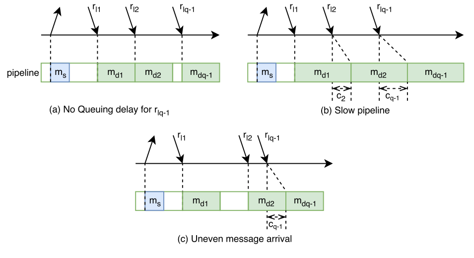
In the case of empty pipeline, the message exits the queue at time \(t_{fi} = t_{ei} + o\), where \(o\) is message processing overhead \(m_s\) or \(m_d\) depending on whether the message is outgoing or incoming. However, if there is a message in the queue already, then the processing of \(l_i\) will stall or clog for some queue waiting time \(w_i\), thus it will exit the pipeline at time \(t_{fi} = t_{ei} + w_i + o\). To compute \(w_i\) we need to know when message \(l_{i-1}\) is going to leave the queue: \(w_i = t_{fi-1} – t_{ei}\). In its turn, the exit time \(t_{fi-1}\) depends of \(w_{i-1}\), and so we need to compute it first. We can continue to “unroll” the pipeline until we have a message \(l_n\) without any queue waiting time (\(w_{i-n} = 0\)). We can compute the dequeue time for that message \(l_n\), which in turns allows us to compute exit time of all following messages. Figure 1 shows different ways a pipeline can get clogged, along with the effects of clog accumulating over time.

Unlike earlier, today I also want to model the overheads of communicating with the clients, since in practice we tend to measure the performance as observed by the clients. This requires the round model to account for client communication latency \(r_c\) which is one network RTT. Each round also adds a single message deserialization (client’s request) and a message serialization (reply to a client) to the queue.

Let me summarize the parameters and variables we need to model the queuing costs:

• \(r_c\) – RTT time to communicate with the client
• \(n_p\) – the number of parallel queues/pipelines. You can roughly think of this as number of cores you wish to give the node.
• \(s_p\) – pipeline’s service rate (messages per unit of time). \(s_p = \frac{N+2}{N\mu_{md} + 2 \mu_s}\)
• \(w_i\) – pipeline waiting time for message \(l_i\)
• \(R\) – throughput in rounds per unit of time.
• \(\mu_{r}\) – mean delay between rounds. \(\mu_{r} = \frac{1}{R}\)
• \(\sigma_{r}\) – standard deviation of inter-round delay.

Now lets talk about some these parameters a bit more and how they relate to the model.

Pipeline service rate \(s_p\) tells how fast a pipeline can process messages. We can get this metric by looking at average latencies of message serialization \(\mu_{ms}\) and deserialization/processing \(\mu_{md}\). With \(N\) nodes in the cluster, we can find an average message overhead of the round \(\mu_{msg}\). For a given round, the leader node needs to handle 2 message serializations (one to start the round and one to reply back to client and \(N\) deserializations (\(N-1\) from followers and one from the client). This communication pattern gives us \(\mu_{msg} = \frac{N\mu_{md}+2\mu_{ms}}{N+2}\). A reciprocal of \(\mu_{msg}\) gives us how many messages can be handled by the pipeline per some unit of time: \(s_p = \frac{N+2}{N\mu_{md} + 2\mu_s}\).

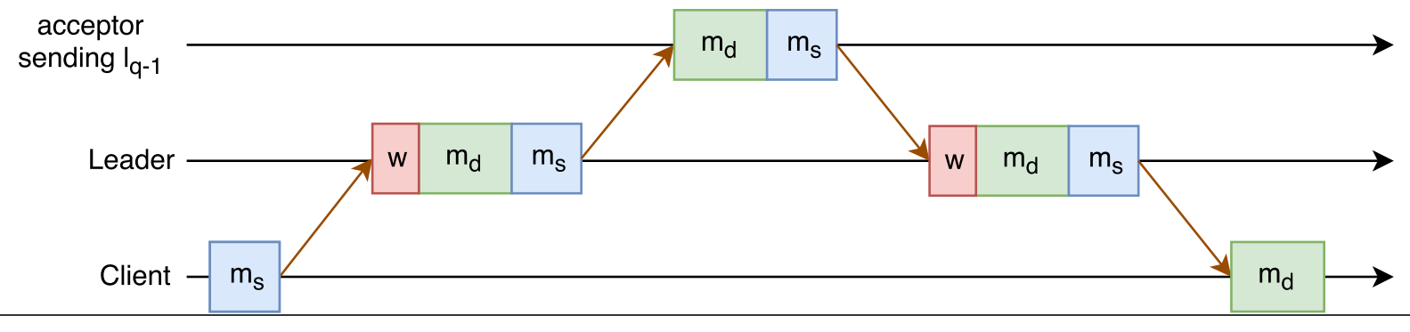
Variable \(w_i\) tells how backed up the pipeline is at the time of message \(l_i\). For instance, \(w_i = 0.002 s\) means that a message \(l_i\) can start processing only after 0.002 seconds delay. Figure 2 illustrates the round execution model with queue wait overheads.

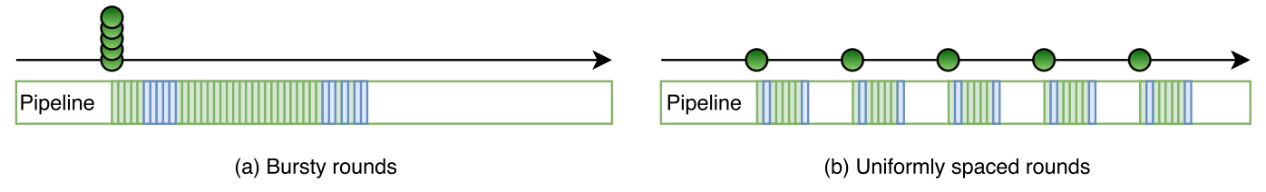
To properly simulate multi-paxos, I need to look at multiple rounds. Variable \(R\) defines the throughput I try to push through the cluster, as higher throughput is likely to lead to longer queue wait times. I also need to take into consideration how rounds are distributed in time. On one side of the spectrum, we can perform bursty rounds, where all \(R\) rounds start at roughly the same time. This will give us the worst round latency, as the pipelines will likely clog more. On the other side, the rounds can be evenly dispersed in time, greatly reducing the competition for pipeline between messages of different rounds. This approach will lead to the best round latency. I have illustrated both of these extremes in round distribution in Figure 3.

However, the maximum throughput \(R_{max}\) is the same no matter how rounds are spread out, and it is governed only by when the the node reaches the pipeline saturation point: \(R_{max}(N+2) = n_ps_p\) or \(R_{max}(N+2) = \frac{n_p(N+2)}{N\mu_{md} + 2\mu_{ms}}\). As such, \(R_{max} = \frac{n_p}{N\mu_{md} + 2\mu_{ms}}\). In the actual model simulation, the latency is likely to spike up a bit before this theoretical max throughput point, as pipeline gets very congested and keeps delaying messages more and more.

The likely round distribution is probably something more random as different clients interact with the protocol independently of each other, making such perfect round synchronization impossible. For the simulation, I am taking the uniform separation approach and add some variability to it by drawing the round separation times from a normal distribution \(\mathcal{N}(\mu_r, \sigma_r^2)\). This solution may not be perfect, but normal distribution tend to do fine in modeling many natural random phenomena. I can also control how much different rounds can affect each other by changing the variance \(\sigma_r^2\). When \(\sigma_r\) is close to 0, this becomes similar to uniformly spaced rounds, while large values of \(\sigma_r\) create more “chaos” and conflict between rounds by spreading them more random.

Now I will put all the pieces together. To model the round latency \(L_r\), I modify the old formula to include the queuing costs and client communication delays. Since the round latency is driven by the time it takes to process message \(l_{q-1}\), I only concern myself with the queue waiting time \(c_{q-1}\) for the quorum message. As such, the new formula for round latency is \(L_r = (m_s + r_{lq-1} + c_{q-1} + m_d) + (m_{cd} + m_{cs} + r_c)\). In this formula, \(m_{cd}\) is deserialization overhead for the client request, and \(m_{cs}\) is the serialization overhead for server’s reply back to client.

Simulation Results

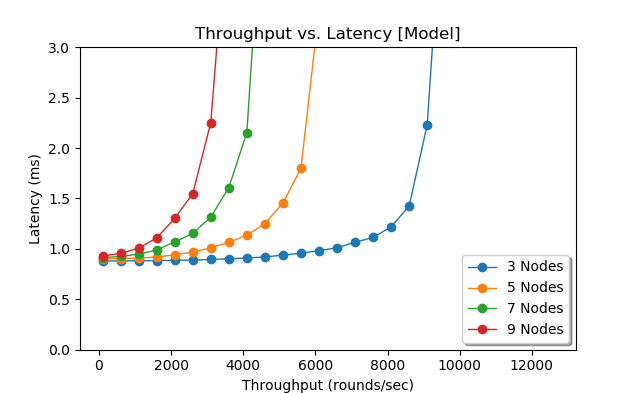
As before, I have a python script that puts the pieces together and simulates multi-paxos runs. There are quite a few parameters to consider in the model, so I will show just a few, but you can grab the code and tinker with it to see how it will behave with different settings. Figure 4 shows the simulation with my default parameters: network settings taken from AWS measurements, pipeline performance taken from the early paxi implementation (now it is much faster). Only one pipeline/queue is used. The distribution of rounds in time is controlled by inter-round spacing \(\mu_r = \frac{1}{R}\) with \(\sigma_{r} = 2\mu{r}\).

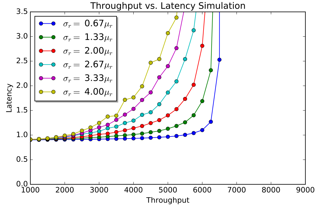
Next figure (Figure 5) shows how latency changes for inter-round delay variances. The runs with higher standard deviation \(\sigma_r\) appear more “curvy”, while the runs with more uniform delay do not seem to degrade as quick until almost reaching the saturation point. High \(\sigma_r\) runs represent more random, uncoordinated interaction with the cluster, which on my opinion is a better representation of what happens in the real world.

Do I Need to Simulate Paxos Rounds?

The results above simulate many individual rounds by filling the pipeline with messages and computing the queue wait time for each round. Averaging the latencies across all simulated rounds produces the average latency for some given throughput. However, if I can compute the average queue waiting time and the average latency for the quorum message, then I no longer need to simulate individual rounds to essentially obtain these parameters. This will allow me to find the average round latency much quicker without having to repeat round formula computations over and over again.

Let’s start with computing average latency for a quorum message \(r_{lq-1}\). Since that \(l_{q-1}\) represents the last message needed to make up the quorum, I can model this message’s latency with some \(k\)th-order statistics sampled from Normal distribution \(\mathcal{N}(\mu_l+\mu_{ms}+\mu_{md}, \sigma_l^2 + \sigma_{ms}^2 + \sigma_{md}^2)\) on a sample of size \(N-1\), where \(k=q-1\). To make things simple, I use Monte Carlo method to approximate this number \(r_{lq-1}\) fairly quickly and accurately.

Now to approximating the queue wait time \(w_{q-1}\). This is a bit more involved, but luckily queuing theory provides some easy ways to compute/estimate various parameters for simple queues. I used Marchal’s average waiting time approximation for single queue with generally distributed inter-arrival and service intervals (G/G/1). This approximation allows me to incorporate the inter-round interval and variance from my simulation into the queuing theory model computation.

I will spare the explanation on arriving with the formula for the average round queue wait time (it is pretty straightforward adaptation from here, with service and arrival rates expressed as rounds per second) and just give you the result for a single queue and single worker:

• \(p = R(N\mu_{md} + 2\mu_{ms})\), where \(p\) is queue utilization or probability queue is not busy.
• \(C_s^2 = \frac{N^2\sigma_{md}^2 + 2^2\sigma_{ms}^2}{(N\mu_{md} + 2\mu_{ms})^2}\)
• \(C_a^2 = \frac{sigma_r^2}{\mu_r^2}\)
• \(w=\frac{p^2(1+C_s^2)(C_a^2+C_s^2p^2)}{2R(1-p)(1+C_s^2p^2)}\)

With the ability to compute average queue waiting time and average time for message \(l_{q-1}\) turn around, I can compute the average round latency time for a given throughput quickly without having to simulate multiple rounds to get the average for these parameters. \(L = 2\mu_{ms} + 2\mu_{md} + r_{lq-1} + w + \mu_l\), where \(r_{lq-1}\) is the mean RTT for quorum message \(l_{q-1}\) and \(w\) is the average queue wait time for given throughput parameters and \(\mu_l\) is the network RTT for a message exchange with the client.

As such, the average round latency becomes:

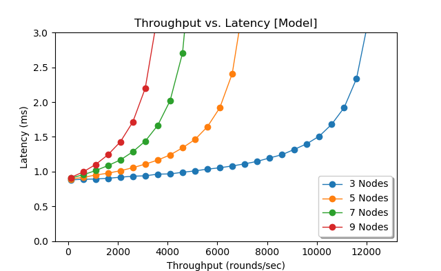
\(L = 2\mu_{ms} + 2\mu_{md} + r_{lq-1} + \frac{p^2(1+C_s^2)(C_a^2+C_s^2p^2)}{2R(1-p)(1+C_s^2p^2)} + \mu_l\)

Figure 6 shows the model’s results for latency at various throughputs. The queuing theory model exhibits very similar patterns as the simulation, albeit the simulation seems to degrade quicker at higher throughputs then the model, especially for 3-node cluster. This may due to the fact that the simulation captures the message distribution within each round, while the model looks at the round as one whole.

Flexible Quorums

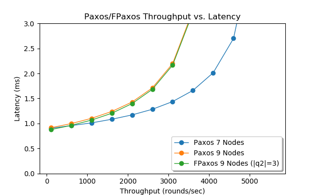
I can use both the simulation and the model to show the difference between paxos and flexible paxos (FPaxos) by adjusting the quorums. For instance, I modeled a 9-node deployment of flexible paxos with phase-2 quorum \(q2\) of 3 nodes. In my setup, flexible paxos must still communicate with all 9 nodes, but it needs to wait for only 2 replies, thus it can finish the phase quicker then the majority quorum. However, as seen in Figure 7, the advantage of smaller quorum is tiny compared to normal majority quorum of 9-node paxos. Despite FPaxos requiring the same number of messages as 5-node paxos setup, the costs of communicating with all 9 nodes do not allow it to get closer in performance event to a 7-machine paxos cluster.

Conclusion and Next steps

So far I have modeled single-leader paxos variants in the local area network. I showed that network variations have a negligible impact on majority quorum paxos. I also illustrated that it is hard to rip the performance benefits from flexible quorums, since queuing costs of communicating with large cluster become overwhelming. However, not everything is lost for FPaxos, as it  can reduce the number of nodes involved in phase-2 communication from full cluster size to as little as \(|q2|\) nodes and greatly mitigate the effects of queue waiting time for large clusters.

The simulation and model are available on GitHub, so you can check it out and tinker with parameters to see how the performance may change in response.

There are still quite a few other aspects of paxos that I find interesting and want to model in the future. In particular, I want to look at WAN deployments, multi-leader paxos variants and, of course, our WPaxos protocol that combines multi-leader, WAN and flexible quorums.