Many, if not all, practical distributed systems rely on partial synchrony in one way or another, be it a failure detection, a lease mechanism, or some optimization that takes advantage of synchrony to avoid doing a bunch of extra work. These partial synchrony approaches need to know some crucial parameters about their world to estimate how much synchrony to expect. A misjudgment of such synchrony guarantees may have significant negative consequences. While most practical systems plan for periods of lost partial synchrony and remain safe, they may still pay the performance or availability cost. For example, a failure detector configured for a very short timeout may cause false positives and trigger unnecessary and avoidable misconfigurations, which may increase latency or even make systems unavailable for the duration of reconfiguration. Similarly, a system that uses tight timing assumptions to remain on an optimized path may experience performance degradation when such synchrony expectations do not hold. One example of the latter case is EPaxos Revisited and their TOQ optimization that uses tight assumptions about communication delays in the cluster to avoid conflicts and stay on the “fast path.”

More recently, the partial synchrony window has been shrinking in systems, with many algorithms expecting timeouts or tolerances of under ten milliseconds. Moreover, some literature proposes schemes that work best with sub-millisecond timing tolerances. However, how realistic are these tight timing tolerances?

Systems use timing assumptions to manage the communication synchrony expectations. For example, failure detectors check whether the expected heartbeat message has arrived in time. Systems relying on synchrony for “fast path” use timing assumptions, explicitly or implicitly, to judge the existence of messages—if nothing has arrived in some time window, then a system may expect that nothing has been sent in the first place. For instance, algorithms like Rabia or EPaxos Revisited TOQ rely on this assumption implicitly, as the protocol expects some message to arrive at all participating nodes at nearly the same time for optimal performance. A node that has not received the message in time will be in a mismatched state and potentially cause a delay when the algorithm needs to check/enforce safety.

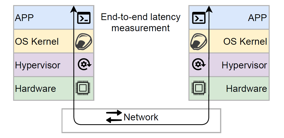
Anyway, to decide whether the tight timing tolerances required by some protocols are realistic, we need to look at what communication latency underlying infrastructure can provide. This communication latency is end-to-end latency between two processes running in different nodes in some infrastructure, such as the cloud. Many factors impact this end-to-end, process-to-process communication latency. Starting from the obvious, the network between nodes plays a major role, but the communication goes through other layers as well, such as virtualization, OS kernel, and even the application/system process itself.

Last semester, in my seminar on the reliability of distributed systems, some students and I did a little experiment measuring this end-to-end latency in various public clouds to see what timing assumptions are realistic. We prepared a report and even tried to publish it twice, but it seems the reviewers do not care about our trivially collected observations (more on this in the “Rant” section at the end).

See, measuring end-to-end latency is not hard. Ping utility does that. So, we wrote a Cloud Latency Tester (CLT), essentially a bigger ping utility that works over TCP sockets, sends messages of configured size at a configured rate across many deployed instances, and finally records the round trip time between all pairs of nodes. CLT works in rounds — each node sends a ping message to all peers and expects the peers to respond with a corresponding pong message carrying the same payload. Each node records the round-trip latency observed for each peer in each ping round. The rounds also allow for the extrapolation of additional information, such as quorum latency.

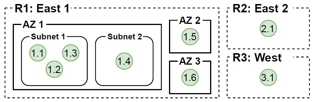
We then deployed CLT in the big three (AWS, Azure, and GCP) on some of their more popular VMs and let it run. For the deployment, we wanted to test some meaningful scenarios, such as latency within the same AZ of a region, across three AZs of a region, and across several cloud regions. The figure illustrates the deployment strategy we followed for all cloud providers. For nodes inside the AZ, we also tried to see if separating them into different subnets made any difference (it did not); hence, some nodes in the same AZ appear in different subnets. And for VM choice, we settled on supposedly popular but small VM instances — all VMs had 2 vCPUs and 8 GB of RAM and similar enough network bandwidth. Finally, we let CLT cook for 6 hours between 2 and 8 p.m. on the weekday at a rate of 100 rounds per second at each node with 1024 bytes of payload.

Below, I summarize our observations and lessons learned. Note that our goal was not to compare the cloud vendors; instead, we wanted to know what engineers can expect from latency between processes — how small or large it is and how predictable it appears. Let’s start with a high-level summary overview:

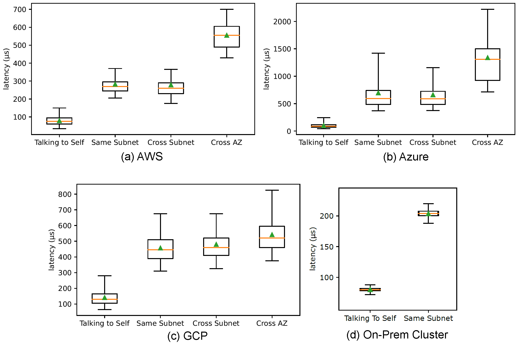
This summary figure illustrates a few things. For one, talking to oneself is not very fast. While it is faster than talking to a process in remote VMs, even that is not always the case. Second, we can expect some decent variability in communication latency. Just a pick at Azure figure shows 95th percentile latency gets closed to 1.5 ms, almost 2× the average latency! Finally, as expected, cross-AZ communication overall is slower in all clouds and tends to have higher variance.

Now, let’s zoom in on each cloud provider. The figure below shows 30-second latency averages for each provider:

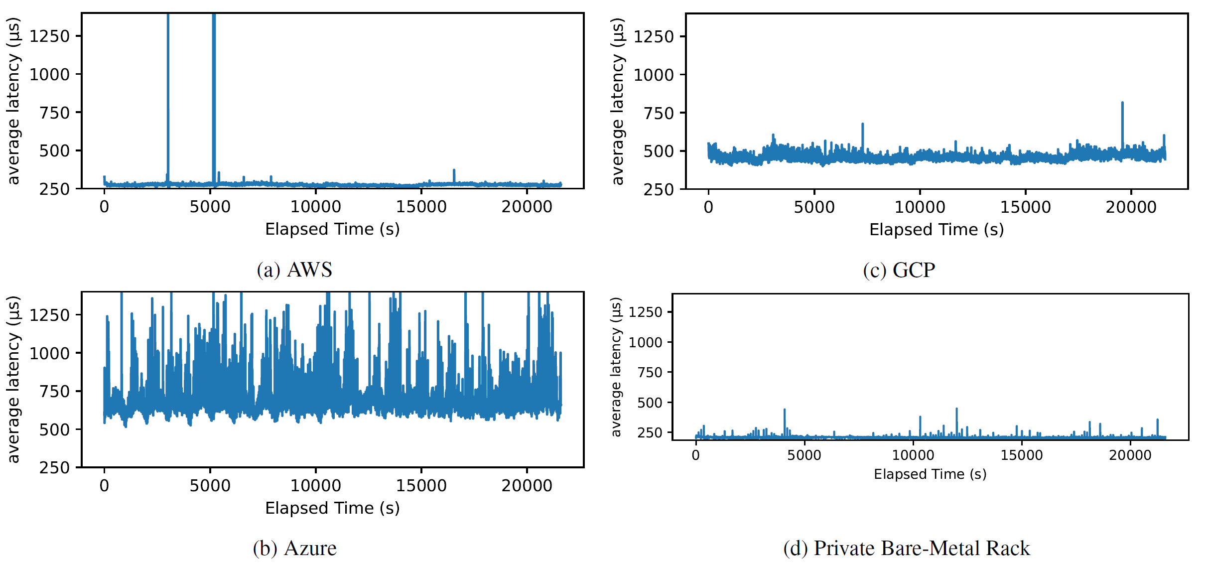
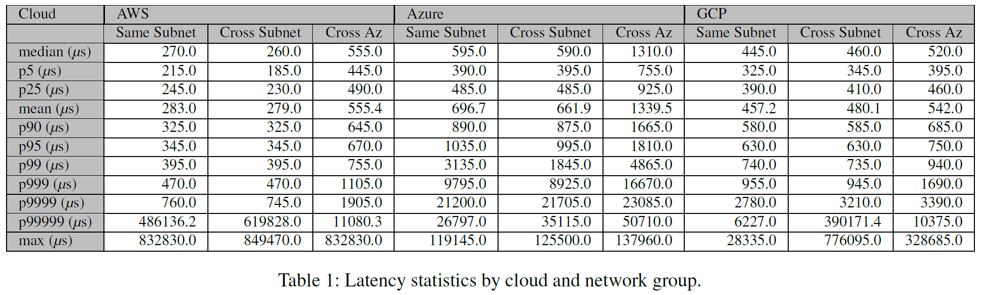
An obvious feature of AWS data is two big latency spikes. While looking at the raw data, the culprit seemed to be a few smaller spikes happening within a few seconds of each other. The highest such spike clocked at 832.83 ms or 2,900× the average latency. It occurred at one node in one communication round for all peers except oneself. Since the loopback communication worked without a problem, we think that the problem was external to the VM. Azure data is very puzzling. Aside from showing frequent spikes above 1 ms for many 30-second windows, the data also suggests the existence of some cyclical pattern with a roughly 20-minute cadence. GCP data seemed the most boring among the three. Finally, we also include a similar measurement on equipment in our lab; to our delight, aside from the few big spikes, AWS data looks similar to what we get in our hardware.

The figure below takes a look at the same latency data, but presents it as a latency histogram and latency CDF:

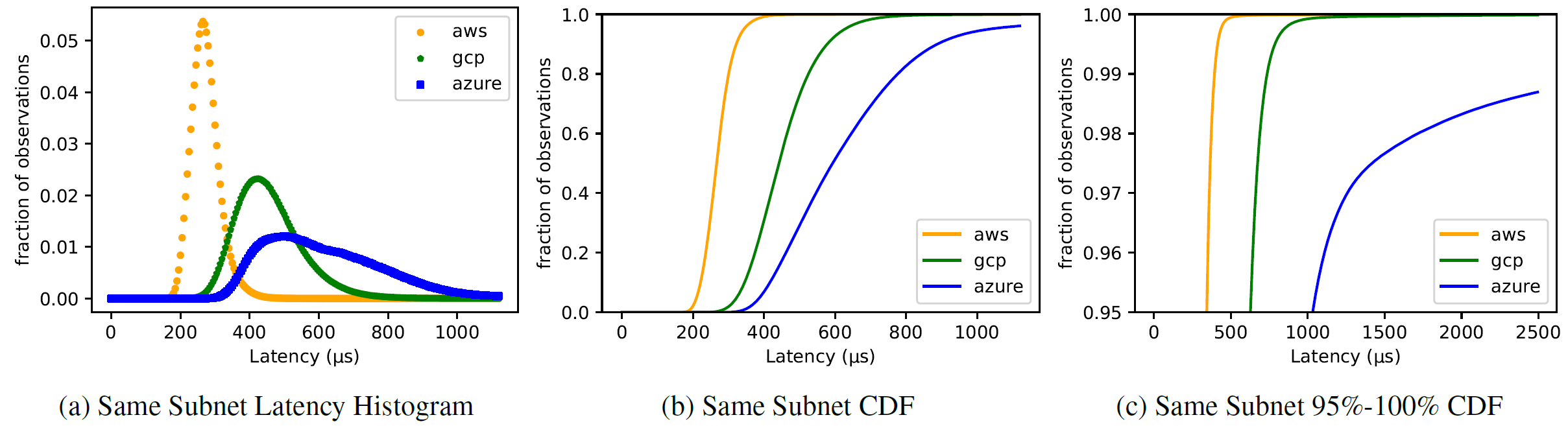
With this figure, we see a lot of interesting stuff. For one, Azure has the longest tail towards high latency that fades very slowly. AWS and GCP seem more predictable in this regard, with observation looking more Normal. The Azure’s tail was so bad, that we had to cut it out from the CDF figure for space reasons — the 99th percentile exceeded 2.5 ms!

The next figure shows latency between individual pairs of nodes in the same subnet of the same AZ:

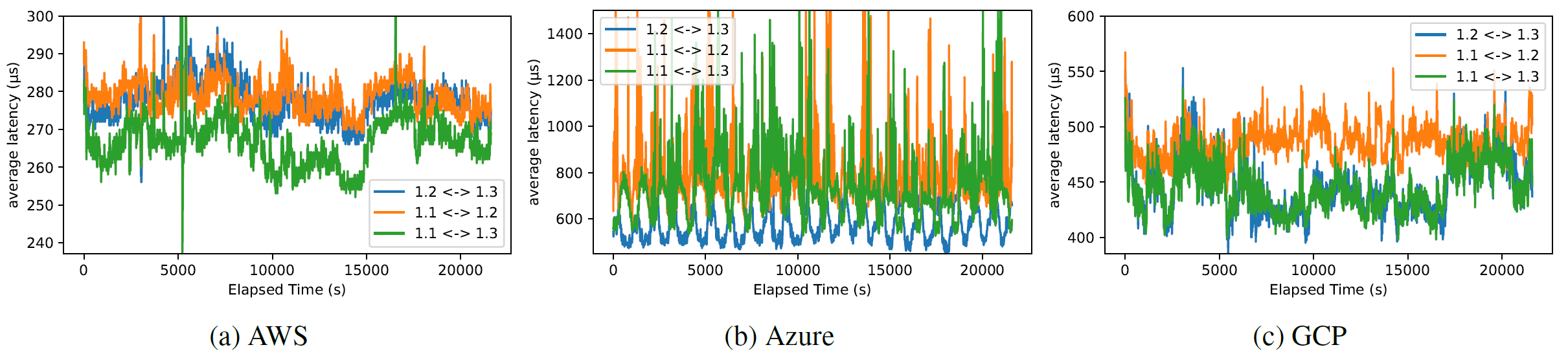
Of the peculiar observations here are the changes in latency that happen over time. For instance, there is a noticeable increase in latency on AWS after 15,000 seconds of run time. On GCP, a similar increase exists but only on some nodes. The cyclical patterns on Azure are more visible in this figure.

Finally, let’s look at some data for talking across AZs:

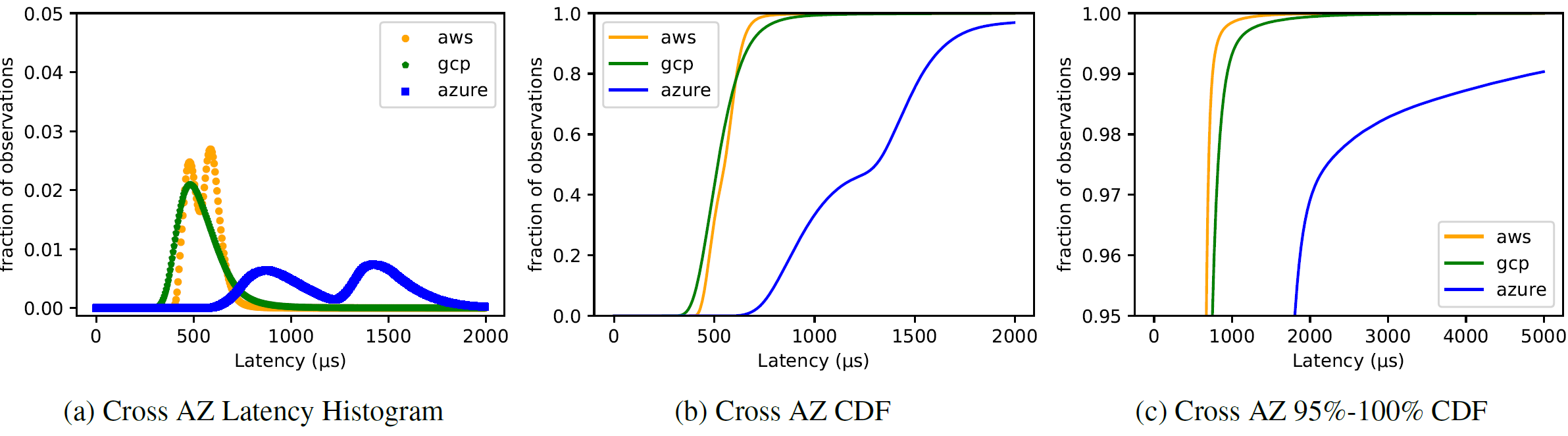
Here we can easily see multi-modal latency distributions — it appears that, at least in AWS and Azure, the latency/distance between AZs is not uniform, which results in different pairs of nodes having different latency. It is worth noting that similar behavior can be observed even within the same AZ — depending on the placement of VMs inside the AZ, some pairs may be quicker than others. I will not put the figure for this, but it is available in the report.

Finally, I want to talk briefly about quorums. Quorums are powerful communication primitives used in many data-intensive protocols. Quourms allow the masking of failed nodes, but also mask the slowest nodes, so looking at quorum latency makes a lot of sense for such systems:

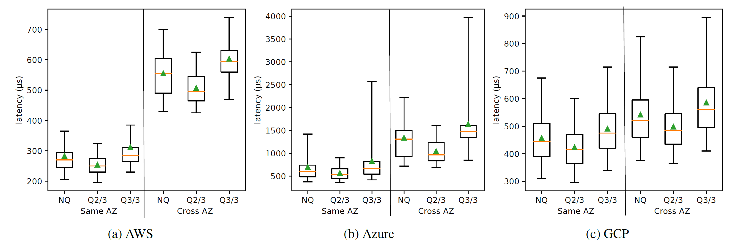
Here, as expected, a quorum of 2 out of 3 nodes appears a bit faster than individual messages or waiting for all peers in the cluster (i.e., a quorum of all nodes captures the worst-case latency). What is missing from the box plots is very extreme tail latency, and this is where quorums excel — at 99.999th percentile, the 2-out-of-3 quorum latency is better than individual message latency by up to 577X in our measurements.

I think I will stop with figures here; the report has more stuff, including the discussion of cross-region latency. Our goal was to see what communication latency one can expect in the cloud, and I think we got some pretty interesting data. The bottom line is that I do not think the general purpose cloud is ready yet for sub-millisecond timing assumptions that a lot of academic literature is pursuing now. There are a few other implications for my academic friends — testing/benchmarking systems in the cloud can be tricky — your latency can noticeably change over time. Also, unless you are careful with node placement (and picking leaders in leader-based systems), that placement can impact latency observations.

Rant Time

This is an observation study that, in my opinion, shows some useful/interesting data for system builders/engineers. This study treats the cloud as a black box, exactly as it appears for cloud users, and measures the end-to-end latency as observed by processes running on different nodes in the cloud. It does not try to break down the individual factors contributing to the latency. While these factors may be very useful for cloud providers and their engineering teams to troubleshoot and optimize their infrastructure, for cloud users, it is irrelevant whether the high latency is caused by the cloud network, virtualization technology, or bad VM scheduling. What matters for cloud users is the latency their apps/systems see, as these latencies also drive the safe timing assumptions engineers can take. I believe this point was one of the reasons the JSys reviewers rejected the report — the reviewers wanted to see the network latency and got the end-to-end one. However, the report clearly states that in the very first figure that shows what exactly we measure.

Of course, this observation study is far from perfect, and several factors could have influenced our observations, such as hidden failures in the cloud providers, using only relatively small VMs, and running only for a few hours. The reviewers, of course, are eager to point out these “problems,” again, despite the report clearly stating these deficiencies. However, running things for longer will not solve the latency variations we already observed in 6 hours. If anything, it will show more stuff and more patterns, such as daily latency fluctuations. Longer runs do not invalidate the plethora of observations we made with just a handful of shorter runs. Similarly, trying with bigger VMs will give more valuable and complete data. Maybe (and likely) bigger VM instances will be more stable. However, smaller instances are still more numerous in the cloud, making our observations valid for many users.

Anyway, the report is now on arxiv, and I am done with this little project.