Modeling Paxos Performance in Wide Area – Part 3

Earlier I looked at modeling paxos performance in local networks, however nowadays people (companies) use paxos and its flavors in the wide area as well. Take Google Spanner and CockroachDB as an example. I was naturally curious to expand my performance model into wide area networks as well. Since our lab worked on WAN coordination for quite some time, I knew what to expect from it, but nevertheless I got a few small surprises along the way.

In this post I will look at Paxos over WAN, EPaxos and our wPaxos protocols. I am going to skip most of the explanation of how I arrived to the models, since the models I used are very similar in spirit to the one I created for looking at local area performance. They all rely on queuing theory approximations for processing overheads and k-order statistics for impact of quorum size.

Despite being similar in methods used, modeling protocols designed for WAN operation proved to be more difficult than local area models. This difficulty arises mainly from the myriad of additional parameters I need to account for. For instance, for Paxos in WAN I need to look at latencies between each node in the cluster, since the WAN-networks are not really uniform in inter-region latencies. Going up to EPaxos, I have multiple leaders to model, which means I also must take into consideration the processing overheads each node takes in its role of following other nodes for some slots. wPaxos takes this even further: to model its performance I need to consider access locality and “object stealing” among other things.

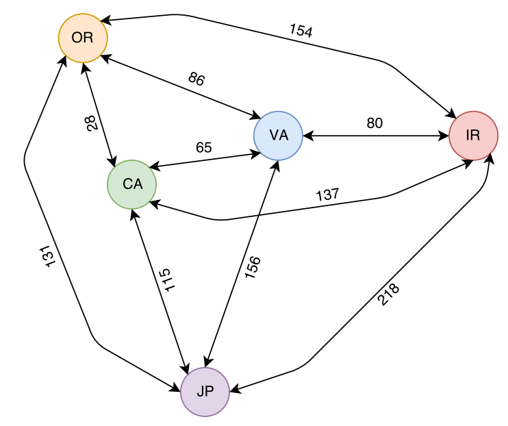
Today I will focus only on 5 region models. In particular, I obtained average latencies between 5 AWS regions: Japan (JP), California (CA), Oregon (OR), Virginia (VA) and Ireland (IR). I show these regions and the latencies between them in Figure 1 below.

Figure 1: Some AWS regions and latencies in ms between them.

Paxos in WAN

Converting paxos model from LAN to WAN is rather straightforward; all I need to do is to modify my paxos model to take non-uniform distances between nodes. I also need the ability to set which node is going to be the leader for my multi-paxos rounds. With these small changes, I can play around with paxos and see how WAN affects it.

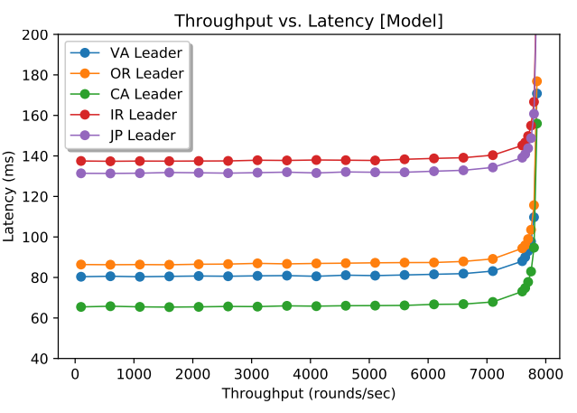
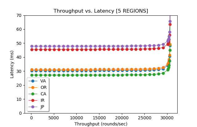
Figure 2 (above) shows a model run for 5 nodes in 5 regions (1 node per region). From my previous post, I knew that the maximum throughput of the system does not depend on network latency, so it is reasonable for paxos in WAN to be similar to paxos in local networks in this regard. However, I was a bit surprised to see how flat the latency stays in WAN deployment almost all the way till reaching the saturation point. This makes perfect sense, however, since the WAN RTT dominates the latency and small latency increases due to the queuing costs are largely masked by large network latency. This also may explain why Spanner, CockroachDB and others use paxos in databases; having predictable performance throughout the entire range of load conditions makes it desirable for delivering stable performance to clients and easier for load-balancing efforts.

However, not everything is so peachy here. Geographical placement of the leader node plays a crucial role in determining the latency of the paxos cluster. If the leader node is too far from the majority quorum nodes, it will incur high latency penalty. We see this with Japan and Ireland regions, as they appear far from all other nodes in the system and result in very high operation latency.

EPaxos

EPaxos protocol tries to address a few shortcoming in paxos. In particular, EPaxos no longer has a single leader node and any node can lead some commands. If commands are independent, then EPaxos can commit them quickly in one phase using a fast quorum. However, if the command have dependencies, EPaxos needs to run another phase on a majority quorum (at which point it pretty much becomes Paxos with two phases for leader election and operation commit). The fast quorum in some cases may be larger than the majority quorum, but in the 5-node model I describe today, the fast quorum is the same as the majority quorum (3 nodes).

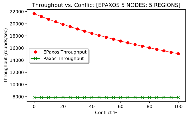
Naturally, conflict between commands will impact the performance greatly: with no conflict, all operations can be decided in one phase, while with 100% conflict, all operations need two phases. Since running two phases requires more messages, I had to change the model to factor in the probability of running two phases. Additionally, the model now looks at the performance of every node separately, and account for the node leading some slots and following on the other.

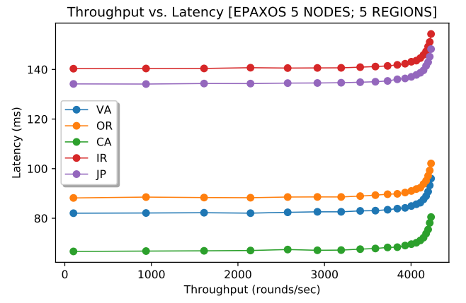
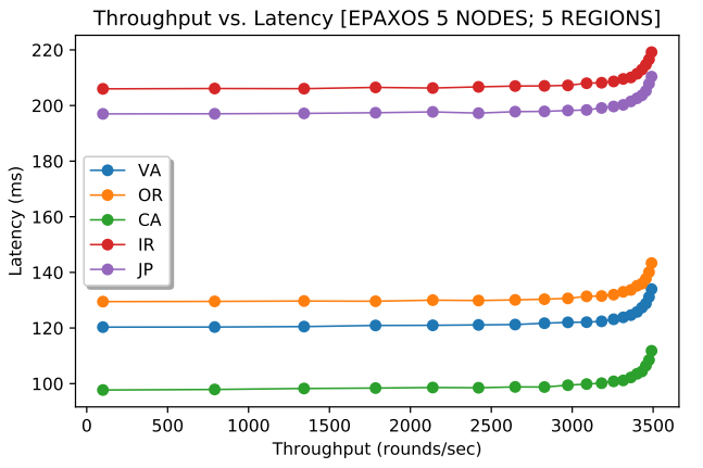
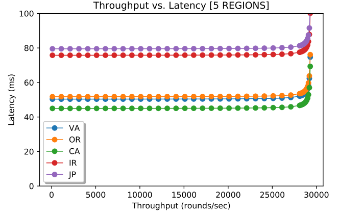
Figure 3: EPaxos throughput at every node with 2% command conflict.

Figure 4: EPaxos throughput at every node with 50% command conflict.

Figures 3 and 4 (above) show EPaxos performance at every node for 2% and 50% conflict. Note that the aggregate throughput of the cluster is a sum of all 5 nodes. For 2% conflict, the max throughput was 2.7 times larger than that of Paxos. As the conflict between commands increases, EPaxos loses its capacity and its maximum throughput decreases, as I illustrate in Figure 5 (below). This changing capacity may make more difficult to use EPaxos in production environments. After all, workload characteristics may fluctuate throughout the system’s lifespan and EPaxos cluster may or may not withstand the workloads of identical intensity (same number of requests/sec), but different conflict.

EPaxos aggregate throughput for different conflict levels. — Figure 5: EPaxos aggregate maximum throughput for different conflict levels.

wPaxos

wPaxos is our recent flavor of WAN-optimized paxos. Its main premise is to separate the commands for different entities (objects) to different leaders and process these commands geographically close to where the entities are required by clients. Unlike most Paxos flavors, wPaxos needs large cluster, however, thanks to flexoble quorums, each operations only uses a subset of nodes in the cluster. This allows us to achieve both multi-leader capability and low average latency.

wPaxos, however, has lots of configurable parameters that all affect the performance. For instance, the fault tolerance may be reduced to the point where a system does not tolerate a region failure, but can still tolerate failure of nodes within the region. In this scenario (Figure 6, below), wPaxos can achieve the best performance with aggregate throughput across all regions (and 3 nodes per region for a total of 15 nodes) of 153,000 requests per second.

Figure 6: wPaxos with no region fault tolerance and 70% region-local operations and 1% chance of object migration.

We still observe big differences in latencies due to the geography, as some requests originating in one regions must go through stealing phase or be resolved in another region. However, the average latency for a request is smaller than that of EPaxos or Paxos. Of course, a direct comparison between wPaxos and EPaxos is difficult, as wPaxos (at least in this model configuration) is not as fault tolerant as EPaxos. Also unlike my FPaxos model from last time, wPaxos model also reduces the communication in phase-2 to a phase-2 quorum only. This allows it to take much bigger advantage of flexible quorums than “talk-to-all-nodes” approach. As a result, having more nodes helps wPaxos provide higher throughput than EPaxos.
Some EPaxos problems still show-up in wPaxos. For instance, as the access locality decreases and rate of object migration grows, the maximum throughput a cluster can provide decreases. For instance, Figure 7 (below) shows wPaxos model with locality shrunken to 50% and object migration expanded to 3% of all requests.

Figure 7: wPaxos with no region fault tolerance and 50% region-local operations and 3% chance of object migration.

How Good Are the Models?

I was striving to achieve the best model accuracy without going overboard with trying to account all possible variables in the model. The models both for LAN and WAN seems to agree fairly well with the results we observe in our Paxi framework for studying various flavors of consensus.

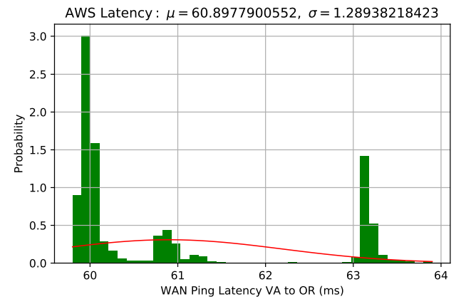
However, there is always room for improvement, as more parameters can be accounted for to make more accurate models. For instance, WAN RTTs do not really follow a single normal distribution, as a packet can take one of many routes from one region to another (Figure 8, below). This may make real performance fluctuate and “jitter” more compared to a rather idealistic model.

Figure 8: WAN Latency between VA and OR.

I did not account for some processing overheads as well. In EPaxos, a node must figure out the dependency graph for each request, and for high-conflict workloads these graphs may get large requiring more processing power. My model is simple and assumes this overhead to be negligible.

Few Concluding Remarks

Over the series of paxos performance modeling posts I looked at various algorithms and parameters that affect their performance. I think it truly helped me understand Paxos a bit better than before doing this work. I showed that network fluctuations have little impact on paxos performance (k-order statistics helps figure this one out). I showed how node’s processing capacity limits the performance (I know this is trivial and obvious), but what is obvious, but still a bit interesting about this is that a paxos node processes roughly half of the messages that do not make a difference anymore. Once the majority quorum is reached, all other messages for a round carry a dead processing weight on the system.

The stability of Paxos compared to other more complicated flavors of paxos (EPaxos, wPaxos) also seems interesting and probably explains why production-grade systems use paxos a lot. Despite having lesser capacity, paxos is very stable, as its latency changes little at levels of throughput. Additionally, The maximum throughput of paxos is not affected by the workload characteristics, such as conflict or locality. This predictability is important for production systems that must plan and allocate resources. It is simply easier to plan for a system delivering stable performance regardless of the workload characteristics.

Geography plays a big role in WAN paxos performance. Despite the cluster having the same maximum throughput, the clients will observe the performance very differently depending on the leader region. Same goes with EPaxos and wPaxos, as different regions have different costs associated with communicating to the quorums, meaning that clients in one region may observe very different latency than their peers in some other regions. I think this may make it more difficult to provide same strong guarantees (SLAs?) regarding the latency of operations to all clients in production systems.

There are still many things one can study with the models, but I will let it be for now. Anyone who is interested in playing around may get the models on GitHub.