Paper Review and Summary

Metastable Failures in Distributed Systems

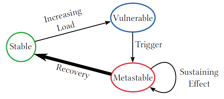
Metastability is a stable state of a dynamical system other than the system’s state of least energy.

Wikipedia

Distributed systems often fail spectacularly and unpredictably. They are a cause for a headache and sleepless on-call nights for way too many engineers. And this is despite lots of efforts to understand the failures, and all the tools and “best practices” we have to contain and/or prevent them. 

Today I want to talk about failures that may occur on a nearly healthy system with no perceived major bugs or design flaws. We describe this type of failure in our HotOS’21 paper. This work is in collaboration with Nathan Bronson, Abutalib Aghayev, and Timothy Zhu. It is largely based on Nathan’s observations and experiences.

So how does a “healthy” system fail? Naturally, something needs to happen for a failure to occur. We call this something a trigger. Lots of things can act as a trigger (GC, network blips, software pushes, configuration changes, load spikes, etc.). Triggers are impossible to avoid in our multi-tenant unreliable systems. 

Triggers cause backlogs or errors and make the system temporarily less happy. In some cases, however, they cause the system to spiral into the abyss and practically halt any useful work or goodput. When the trigger is removed (it was transient, or removed by the engineers), the system does not recover by itself. So we end up in a peculiar situation when the condition that caused a failure is no longer present, all system’s components seem to be functioning correctly, all servers/nodes are up, the code is working, but nothing useful is actually getting done and goodput remains negligible. 

We call this failure pattern a metastable failure, or rather we say that a system has entered a metastable failure state. The culprit behind metastable failures is a sustaining effect that prevents the system from leaving a bad/failed state even after the initial trigger is removed.

To understand more about the importance of triggers and sustaining effects, we need to look at how most distributed systems are deployed. Resource utilization is a major factor for large systems, as achieving better utilization can save a lot of money at scale. This means that systems often have little extra resources to spare when some unexpected load increase occurs. These systems operate in a metastable state that we call a metastable vulnerable state, as the system is vulnerable to a failure if enough of a trigger disturbs its stability.

Of course, having some unanticipated extra load applied to the system is not sufficient for a metastable failure to occur. In fact, even if the load pushes the system to run at its maximum capacity (or tries to run above the capacity), we should only see an increase in latency, and maybe some goodput degradation. When the extra load is removed, the system should return back down to normal operation all by itself. 

In metastable failure, the extra unanticipated load activates a positive feedback loop that creates more load. This positive feedback loop is the sustaining effect that prevents the system from recovering when the initial trigger is resolved. We say that a system is in a metastable vulnerable state when it is possible to activate such a sustaining effect loop using a strong enough trigger. This state typically occurs at the higher system utilization, as the system has fewer spare resources to absorb the extra load of the trigger without activating the positive feedback mechanism. Opposite of metastable vulnerable state is a stable state, where the positive feedback loop is not possible, allowing the system to recover by itself when the extra load is removed. Note that a system in a stable state may still have a sustaining effect mechanism, but it is not strong enough to feed on itself and diminishes over time when the extra load is removed. 

Let’s look at a hypothetical idealized example of a metastable failure. Consider a web application that uses a database capable of serving up to 300 queries per second (QPS). If more than 300 QPS are tried, the latency goes up by an order of magnitude, causing the web application to retry once after a 1-second timeout (when a retry fails, the system errors out). The web servers for the application produce a 280 QPS workload, which falls nicely below the database’s serving capacity.

Now let’s say there was a network glitch lasting a few seconds between the web servers and the database. After the network is fixed, all the delayed packets reach the database, resulting in a flooding manner, exceeding the database’s capacity of 300 QPS. This, in turn, increases the latency above the retry threshold at the web application, causing any new, post-network-glitch queries to retry as well. So now we have a backlog of queries from the network glitch and an effective new query load of 560 QPS (280 queries from the workload + 280 query retries). With such a high and sustained load, the database will not return to a normal state all by itself. This results in a maxed-out system that clears 300 QPS of load (smaller than the amplified load) and produces very little goodput since most of the queries take too long to process and get timed-out or discarded by the time the database returns them. This can continue indefinitely until either the offered workload reduces to under 150 QPS or a retry policy is changed/suspended.

Our simple example illustrates key metastable concepts and principles. In a stable state, a system can (gradually) return to normal operation. In the example, workload under 150 QPS is stable, since even with the workload amplification caused by the retry policy, the database will receive fewer new requests than it can handle each second, allowing it to gradually clear up the backlog and return to normal operation. While the system is clearing the backlog, its goodput, however, may remain compromised. Systems often operate in the vulnerable state because it seems from all metrics like the stable state is wasting resources, and the vulnerability is not known. This, however, leaves very little spare resources to absorb the extra load spikes caused by the trigger events. Once a system enters into a metastable failure state, it will feed onto itself until there is some sort of intervention. This intervention is costly, as it generally requires either reducing the offered load on the system or finding ways to break the positive feedback loops.

Another possible intervention approach is to increase the capacity of the system to push it into a stable state, but this can be challenging since the triggers are unanticipated. Such unpredictability makes it impossible to reconfigure to add capacity beforehand. And once the system is already in a metastable failure state, it may not have any resources to spare to run the reconfiguration procedure. In fact, a reconfiguration may even increase the workload amplification and make the whole situation worse.

In the paper, we discuss a few other hypothetical and anecdotal scenarios that are a bit more complicated. But the problem is not anecdotal by any means, as there are quite a few failure cases that surely look a lot like metastable failures “in the wild”:

  • Google App Engine Incident #19007. Trigger: Configuration change. Sustaining Effect: cascading load amplification. Fix: Reduce traffic level.
  • Amazon SimpleDB Service Disruption. Trigger: power loss crashing multiple servers. Sustaining Effect: load amplification due to a timeout. Fix: Change in timeout policy & introduction of additional capacity.
  • Cassandra Overload because of hint pressure + MVs. Trigger: rolling restart. Sustaining Effect: Few nodes could not catch up with hinted hand-off, preventing them from fully joining, causing the system to generate more hints. Fix: Policy change – disable hinted handoff.

With metastable failures affecting real systems, we need to have more understanding of the problem and processes involved to develop better coping and prevention strategies. A recurring pattern in our experience is that changes meant to improve the common case behavior of a system tend to increase the strength of the sustaining effects. Fast paths, caches, retries, failover, load balancing, and autoscaling all make the failure state less resource-efficient relative to the normal state, which makes the feedback loop worse. Beware of very high cache hit rates!

Metastable failures are over-represented in large site outages because the strength of the sustaining effect depends on scale. For example, if the feedback loop requires overloading a network fabric then small-scale stress tests will never trigger it. The sustaining effect may also act as a means of contagion so that the problem spreads across machines or shards. This means that the first occurrence of a novel metastable failure may be a major outage even in a hyper-scale distributed system.

Current approaches for handling metastability often lack the full comprehension of the problem and its causes. For example, engineers often focus on the trigger that causes the failure and fail to realize the complicated positive feedback loops that are responsible for the scale of the failure. Fixing a trigger is a temporary solution that may only push the system higher into the metastable vulnerable zone and make the next crash even more severe.

Unfortunately, replicating the failures and feedback loops is difficult, as many of the issues only manifest themselves at scale. This makes it ever so harder to fully understand the failures and develop efficient techniques for dealing with them. Furthermore, predicting the possibility of failure is difficult too. For instance, one can look for unexpected performance variations, and try to correlate them with other things going on in the system to learn the potential future triggers, but this still does not give the full predictive power of when a failure may happen. Improvements in our ability to predict and avoid metastable failures will also translate directly to efficiency gains because it will let us operate systems closer to their natural performance limits.

I think this is an exciting area for research. As the industry makes bigger and bigger systems and pushes them to work as cheaply as possible, we need to develop a proper understanding of how these critical systems fail at scale so we can continue improving the reliability.

Paper Summary: Bolt-On Global Consistency for the Cloud

lat1
Figure 1. Latency improvement from going multi-cloud. Minimum read latency SLO feasible when using a single provider for data storage versus when using multiple providers.

This paper appeared in SOCC 2018, but caught my Paxos attention only recently. The premise of the paper is to provide strong consistency in a heterogeneous storage system spanning multiple cloud providers and storage platforms. Going across cloud providers is challenging, since storage services at different clouds cannot directly talk to each other and replicate the data with strong consistency. The benefits of spanning multiple clouds, however, may worth the hustle, since a heterogeneous system will be both better protected from cloud provider outages, and provide better performance by placing the data closer to the users. The latter aspect is emphasized in the paper, and as seen in the figure, going multi-cloud can reduce latency by up to ~25%.

Figure 2. Comparison of (a) classic Paxos and (b) CPaxos.

To solve the issue of consistent cross-cloud replication, authors propose to use Cloud Paxos (CPaxos), a Paxos variant designed to work with followers supporting a very minimal and common set of operations: get and conditional put. In CPaxos, clients act as prospers, and storage systems serve the role of the followers. The followers are not really “smart” in this protocol, and most of the Paxos logic shifts to the client-proposers (Figure 2).

The prepare phase in CPaxos simply gathers the state from the followers, making the proposer decide for itself whether the followers would have accepted it with the current ballot or not. If the proposer thinks it would have been accepted, it will try updating the followers’ state. Doing this, however, requires some precautions from the followers, since their state may have changed after the proposer made a decision to proceed. For that matter, CPaxos uses conditional put (or compare-and-set) operation, making the followers update their state only if it has not changed since it was read by the proposer. This ensures that at most one proposer can succeed with changing the state of the majority of followers.

Figure X. Object log. Each slot corresponds to some version, and can be committed at some ballot #.
Figure 3. Object log. Each slot corresponds to some version, and can be committed at some ballot #.

I visualize this as a log to represent changes in some object’s state. The new version of an object corresponds to a new slot in the log, while each slot can be tried with different ballot by different proposers. The put operation succeeds at the follower only if the value at the slot and a ballot has not been written by some other proposer. In case a proposer does not get a majority of successful updates, it needs to start from the beginning: increase its ballot, perform a read and make a decision whether to proceed with state update. Upon reaching the majority acks on state update, the proposer sends a message to flip the commit bit to make sure each follower knows the global state of the operation.

This basic protocol has quite a few problems with performance. Latency is large, since at least 2 round-trips are required to reach consensus, since every proposer needs to run 2 phases (+ send a commit message). Additionally, increasing the number of proposers acting on the same objects will lead to the growth in conflict, requiring repeated restarts and further increasing latency. CPaxos mitigates these problems to a degree. For example, it tries to commit values on the fast path by avoiding the prepare phase entirely and starting an accept phase on what it believes will be next version of an object with ballot #0. If the proposer’s knowledge of the object’s state (version, ballot) is outdated, the conditional put will fail and the proposer will try again, but this time with full two phases to learn the correct state first. However, if the proposer is lucky, an update can go in just one round-trip. This optimization, of course, works only when an object is rarely updated concurrently by multiple proposers; otherwise dueling leaders become a problem not only for progress, but for safety as well, since two proposers may write different values for the same version using the same ballot. This creates a bit of a conundrum on when the value becomes safely anchored and won’t ever get lost.

Figure 3. Dueling leaders both start opportunistic accept with ballot #0, each writing their own values (green and blue)
Figure 4. Dueling leaders both start opportunistic accept with ballot #0, each writing their own values (green and blue)

Figure 4. Which value to recover in case of the failure? Both green and blue are on the same ballot and have the same number of live nodes
Figure 5. Which value to recover in case of the failure? Both green and blue are on the same ballot and have the same number of live nodes

Consider an example in which two proposers write different values: green and blue to the same version using ballot #0 (Figure 4 on the left). One of the proposers is able to write to the majority, before it becomes unresponsive. At the same time, one green follower crashes as well, leading to a situation with two followers having green value and two being blue (Figure 5 on the right). The remaining proposer has no knowledge of whether the green or blue value needs to be recovered (remember, they are both on the same ballot in the same slot/version!). To avoid this situation, CPaxos expands the fast path commit quorum from majority to a supermajority, namely \(\left \lceil{\frac{3f}{2}}\right \rceil  +1\) followers, where \(2f+1\) is the total number of followers, and f is the tolerated number of follower failures, allowing the anchored/committed value to be in a majority of any majority of followers exploding-head. Having this creates an interesting misbalance in fault tolerance: while CPaxos still tolerates \(f[\latex] node failures and can make progress by degrading to full 2 phases of the protocol, it can lose an uncommitted value even if it was accepted by the majority when up to [latex]f\) followers fail.

Figure 5. (a) messages are sent at the same time; delivery time is different increasing the duration of inconsistency/conflicting state. (b) some messages are sent with delay to provide similar arrival time and reduce the duration of inconsistent state
Figure 6. (a) messages are sent at the same time; delivery time is different increasing the duration of inconsistency/conflicting state. (b) some messages are sent with delay to provide similar arrival time and reduce the duration of inconsistent state

Proposer conflicts are a big problem for CPaxos, so naturally the protocol tries to mitigate it. The approach taken here reduces the duration in which possible conflicts may occur. As CPaxos is deployed over many datacenters, the latencies between datacenters are not likely to be uniform. This means, that a prepare or accept messages from some proposer reach different datacenters at different times, creating an inconsistent state. When two proposers operate concurrently, they are more likely so observe this inconsistency: as both proposers quickly update their neighboring datacenters, they run the risk of not reaching the required supermajority due to the conflicting state (Figure 6(a)) created by some messages being not as quick to reach remaining datacenters. To avoid rejecting both proposers, CPaxos schedules sending messages in a way to deliver them to all datacenters at roughly the same time. This reduces the duration of inconsistent state, allowing to order some concurrent operations (Figure 6(b)).

Figure 6. Degradation in write throughput under different conflict rates.
Figure 7. Degradation in write throughput under different conflict rates.

Despite the above mitigation strategy, conflicts still affect CPaxos greatly. The authors are rather open about this, and show their system CRIC with CPaxos degrading quicker than Paxos and Fast Paxos as the conflict rate increases. However, in the low conflict scenario, which authors argue is more likely in real world applications, CRIC and CPaxos improve on performance compared to Paxos/Fast Paxos, especially for reading the data. This is because reads in CPaxos are carried out in one round-trip-time (RTT) by client-proposer contacting all followers and waiting for at least a majority of them to reply. If the client sees the latest version with a commit flag set in the majority, it can return the data. Otherwise, it will wait to hear from more followers and use their logs to determine the safe value to return. In some rare cases when the proposer cannot determine the latest safe value, it will perform the recovery by running the write path of CPaxos with the value to recover (highest ballot value or highest frequency value if more than one value share the ballot).

Figure 7. Read and write latency.
Figure 8. Read and write latency.

Some Thoughts

  • The motivation of the paper was to make strongly consistent system spanning multiple clouds providers and storage systems for the benefit of improved latency though leveraging the location of datacenters of these different providers. However, CRIC and CPaxos protocol requires a lot of communication, even on the read path. During reads, a client-proposer contacts all CPaxos nodes, located at all datacenters, and in best case still needs the majority replies. As such the latency benefit here comes from trying to get not just one node closer to the client, but a majority of nodes. This may be difficult to achieve in large systems spanning many datacenters. I think sharding the system and placing it on subset of nodes based on access locality can benefit here greatly. For instance, Facebook’s Akkio paper claims to have significant reduction in traffic and storage by having fewer replicas and making data follow access patterns. In our recent paper, we have also illustrated a few very simple data migration policies and possible latency improvement from implementing these policies.
  • One RTT reads in “happy path” can be implemented on top of regular MutliPaxos without contacting all nodes in the systems. Reading from the majority of followers is good enough for this most of the time, while in rare circumstances the reader may need to retry the read from any one node. More on this will be in our upcoming HotStorage ’19 paper.
  • The optimization to delay message sending in order to deliver messages at roughly the same time to all nodes can help with conflict reduction in other protocols that suffer from this problem. EPaxos comes to mind right away, as it is affected by the “dueling leaders” problem as well. Actually, CPaxos and EPaxos are rather similar. Both assume low conflict rate to have single round trip “happy path” writes and reads. When the assumption breaks, and there is a conflict, both switch to two phases. EPaxos is better here in a sense that the first opportunistic phase is not totally wasted and can be used as phase-1 in the two phase mode, whereas CPaxos has to start all the way from the beginning due to the API limitation on the follower side.

Looking at State and Operational Consistency

Recently I rediscovered the “The many faces of consistency” paper by Marcos Aguilera and Doug Terry. When I first read the paper two years ago, I largely dismissed it as trivial, and, oh boy, now I realized how wrong I was at that time.  It is easy to read for sure, and may appear as some summary of various consistency models at first, but it is thought provoking and really makes you ask more questions and draw interesting parallels after giving it some quality time.

Murat gave a good summary of this paper recently in relation to his sabbatical. The questions he asks after the summary, however, provoke even more thoughts about consistency and how we classify, categorize and view it.

In a nutshell, the paper talks about consistency from different perspectives, namely state consistency as observed by a system itself and operational consistency that clients see. State consistency involves enforcing a system-state to hold some invariants. State consistency promotes invariant-based reasoning. The operational consistency is different, as it looks at the system from the client point of view. Outside clients do not directly observe the state of the system, instead they perform operations against it and can only see the results of these operations. So in short, state consistency is invariant-based and concerns with the internal state of the systems. Operational consistency deals with what clients observe from the outside of the system. These operational consistencies include various types sequential equivalence, such as linearizability and serializability, and other client-centric guarantees, like read-your-write or bounded-staleness.

For more details, read the original paper, Murat’s summary or one from the morning paper.

“Strength” of state consistency.

What strikes me right away is how different the two types of consistency are described. Operational consistency gives us the framework for reasoning about systems without having too many details about the internals. We can gauge the relative “strength” of different consistency models and put them in perspective against each other. We know the serializability is weaker then session serializability. Or that linearizability is stronger than sequential equivalence.

But what about state consistency? There is no such reasoning framework. And in fact, it is not easy to even classify state consistency, yet along reason about the “strength” of different state consistency classes. The paper mentions a few state consistency models, such referential integrity for databases, or mutual consistency in primary-backup systems, or error bounds. But these are not generally applicable across the board. These examples of state consistency operate within the constraints of their specific domains or applications.

However, state consistency still comes at different “strength” levels. When reasoning about state consistency, we use invariant-based approach. The invariants on the state we need to enforce for an eventually consistent data-store and a strongly-consistent one are different. In the former case, we can be more relaxed, since we only need to make sure that at least one future state will have different nodes of the store to have the same data. The latter case is more complicated, as we need to hold stricter invariants (i.e. no two alive nodes have different committed value for the same slot in the log, and there can be only one active leader, and the leader must process the commands in the receive order, etc.).

It is the “tightness” of the invariants that makes state consistency strong or weak. But deciding which invariant is tighter or stricter is hard. We cannot simply compare various invariants on the merits of when they should hold, or how many parameters they cover or how many nodes they span, as all these (and other) metrics mean something only in the context of their systems/problems. Invariant that must hold at every state is not necessarily tighter than the eventual one, as it may simply be an invariant against some irrelevant or trivial parameter that holds all the time anyway and has no impact on the system.

And this is why we often translate these invariants and state consistency they represent into the operational consistency. The operational side of things allows us to observe the impact of the invariants on the system, albeit indirectly. Operational consistency levels the playing field and enables the comparison from the external point of view. It allows us to gauge how otherwise hard-to-compare invariants at the state-consistency level affect the outcome of operations.

Smart systems or smart clients

Does this mean that a system providing stronger operational consistency has stronger state consistency? Well, it would have been too simple if that was the case. It often happens, and more so recently, that systems have “misalignments” between their internal state consistency and the operational one exposed on the client side.

A system that provides stronger operational semantics may do so because it has a strong state that makes it easy to expose the strong operational consistency. These smart systems preserve strong state-consistency at all costs. They may need to run complicated algorithms (i.e. Paxos) to achieve that, but doing so makes the clients lean and simple with minimal or no state at all.

On the other hand, simple systems may forgo the complicated protocols needed to enforce a strong state. Instead they aim to run as lean as possible at the core system level and shift as much burden to the smart clients. These clients need to have more complex state and protocols if they are to provide stronger operational guarantees. There are systems that do exactly that.

Both “smart system – lean client” and “lean system – smart client” approaches have their advantages and drawbacks. Designing and maintaining a smart system may actually be simpler: all the things engineers need are readily available at the system level. Invariant-based reasoning and tools like TLA easily apply in this setting. Debugging is simpler too, since lean and stateless clients are likely not the cause of a problem, and internal logging can help collect all the necessary information. On the other hand, having a lean system may improve the performance by reducing the bottlenecks, spreading load more evenly across the nodes and even sharing the load with smart clients. But it comes at some engineering costs. Protocols now involve more state and state is even more distributed: both at the lean system nodes and smart clients. Modeling this state with TLA is still possible, but it will likely take more time to check and require a more complicated models that include clients and client interactions with the system nodes. Debugging may be slowed down due to the lack of necessary data, since many issues (especially on production) may happen at smart clients outside of the engineers’ reach.

Instead of Conclusion

State consistency is an interesting beast. It does not give us the same mental reasoning framework as operational consistency. We, the distributed systems people, often think about the consistency in operational terms. It is easy to understand why, since operational consistency allows for comparison between systems or protocols. But then we, the distributed systems people, also think in terms of state consistency. We model our systems at the state level, trying to give good invariants, try to see what states should always hold, or how a system needs to converge to certain states.

But now understand that there is no clear path from strong state to strong operational consistency. Strong state makes it easier to build operationally strong systems, but it is not a requirement. In fact, for example ZooKeeper, despite having a Paxos-like protocol at its heart is not all that operationally strong. And some systems, like TAPIR or OCCULT, may have weaker state, but with clever engineering and smart clients can provide stronger operational semantics. The world of distributed systems is not black-and-white. There are lots of gray in between.

Is Java Fast Enough for Distributed Applications?

Lots of modern distributed systems are built with Java programming language, and consequently use Java Virtual Machine (JVM) as their execution environment. The list of such systems is rather large: Hadoop, Spark, HBase, Cassandra, Voldemort, ZooKeeper, BookKeeper, Kafka, and the list goes on and on. But is JVM fast enough for these systems?

Anyone who has ever dealt with Java probably knows at least a little bit about how JVM works. To start with, Java programs are compiled into a machine independent, un-optimized byte code. The byte code is then being interpreted by the JVM and compiled into the native code with the just-in-time (JIT) compiler. JVM adds various optimizations at the JIT compilation and these optimizations can be more aggressive than the optimizations done by a native compilers. After all, before doing these optimizations and compilation, Java has already ran the code in the interpreted mode, and it was able to collect some statistics on the branch predictions, loops and function calls to make optimization tailored not just to that specific code, but also to the specific runtime or data.

However, before Java performs all the tricks, it needs to run in a slow interpreted mode, incurring some warm-up overheads. OSDI’16 paper “Don’t Get Caught in the Cold, Warm-up Your JVM” goes into more details about what are the warm-up overheads and how they impact data-parallel distributed systems, such as Hadoop, Spark and Hive.

Warm-up Costs

The paper breaks down warm-up overheads into the two categories: class loading and bytecode interpretation overheads. It investigates these overheads under different workloads on different distributed systems. Of course it is expected for warm-up to impact the freshly started JVM, but how big is the cost of warm-up? If we look at the HDFS client performance, we can see the warm-up can easily take a few seconds, depending on your task. In HDFS, writing is more complicated and involves more classes, thus Java spends more time loading all the classes.  Warm-up while reading from HDFS also differs depending on whether we read in parallel or sequentially. The graph below shows warm-up costs by the task and dataset size.

Figure 1
JVM warm-up overheads. “cl” stands for class loading. “int” is bytecode interpretation.

We can see that the size of the operation has no impact on the overheads, meaning that small operations will spend much larger fraction of their time in warm-up, while big operations tend to amortize the warm-up costs.

figure2
Warm-up overhead as a fraction of total runtime.

It is also interesting to see when the warm-up occurs in the execution cycle. Obviously starting the client requires lots of class loading and interrupting the byte code, however starting actual jobs (for the first time?) also incurs warm-ups.

Figure 3
Warm-up at different execution stages.

Another question one may ask is how slow actual class loading is? For HDFS sequential read, client had to load about 2000 classes, taking 1028 ms to complete.  Spark was much heavier on the classes it uses and needs to load with 19,066 classes on average taking roughly 6.3 seconds in overheads.  These are rather large numbers, especially if we aim at low-latency execution of our requests, however not everything is so grim.

It is important to emphasize that the paper mainly uses clients to study the warm-up, while the actual distributed system is not being studied in much of the details. To be fair, authors mention that the warm-up overheads are present on the server side as well, and in Spark the executor warm-up can add up to almost 50% of the overall warm-up time.

figure4
Spark warm-up overheads.

Dealing with Warm-up

The paper argue that these are very big overheads that must be dealt with. Authors even offer a prototype solution, a modified JVM, called HotTub, which acts as a container for many other “normal” JVMs to be reused when needed. Reusing JVM means we do not need to load classes and perform JIT. Such approach works well for short lived JVMs, i.e we have a client performing one operation and terminating. If such terminated JVM ends up in the pool for JVM reuse, we can save time on overheads next time we need another short-lived JVM.

I have to disagree, however, that these overheads are a big problem, and here is why. JVM running server side of the distributed system are warmed-up if they ran for at least some time. As such, these machines do not experience warm-up costs anymore. In this breakdown of the HDFS request, we do not see any warm-up losses occurring on the data-node side and all of the overheads were due to the warm-up of a short-lived HDFS client. This means that keeping you JVM alive and designing your workloads/client to stay up is the best solution to overcome these type of overheads.

Figure 5
HDFS warm-up.

There are few lessons I have learned from this paper. They may sound like a common sense, but nevertheless these are important points to keep in the back of your head to get the most out of your Java code.

  • Keep JVMs alive. Long running JVMs do not incur as many new class loads and do not need to interpret as much code, allowing the JVM to be faster.
  • Simpler is better. Too Many classes hurt performance on the warm-up, however do not go to extreme on the other side too. After all these are warm-up costs and not constant penalty to your performance.
  • Watch your external libraries. This goes together with previous point. Bringing a big library to perform one small task may not be too wise if similar-performing alternatives are available.

Gorilla – Facebook’s Cache for Time Series Data

Facebook operates a huge infrastructure that needs to be constantly monitored for performance and stability. Such monitoring collects huge amounts of data that must be easily accessible to various diagnosis and anomaly detection tools in order to quickly identify and react to possible issues. Many of such parameters can be represented as real-valued time series. For example, server CPU utilization can be thought of as one of such time series: it can be sampled at some time interval and represented as a numeric value. In order to accommodate all the time series data for various parameter produced by all the server, Facebook needs a scalable, robust and fast way to store and manage time series.

Gorilla: A Fast, Scalable, In-Memory Time Series Database paper describes Facebook’s approach to the problem of managing large amounts of time series. After reading the first page of this paper, I started to ask myself whether Gorilla is truly a time series database or if it is a monitoring data cache for Facebook. To understand what is Gorilla, we must look at what data Gorilla stores and how it was designed and implemented.

Facebook’s monitoring tasks set a strict set of requirements a time series database needs to meet, which I briefly summarize in the list below:

  • Store real-valued monitoring data
  • Have fast access to 26 hours of monitoring data
  • Be scalable on Facebook scale, as the amount of data increases all the time
  • Maintain millions of time series
  • Fast retrieval of time series with reads in under 1 ms
  • Support up to 40,000 queries per second
  • Low granularity time series with resolution of up to 4 data point per second.
  • Replicated design for disaster recovery.

Gorilla Data Model

Gorilla is said to store time series data in which every data point consists of a timestamp and a single 64-bit value. This places the limitation on what kind of time series can be stored. For one, timestamp requirement makes it more difficult to deal with ordinal time series in which only the order of events matters and not the duration between them (sure, we can assign always increasing integers for timestamp to represent the order). Another limitation is inability to store multi-dimensional time series, where a single data point consists of a vector rather than a single value.

Physical time of the event is important for Facebook’s usage case of Gorilla, as the engineers need to know the time when an event or anomaly happened. Facebook engineers also do not care about recording vectors of data for each point in time, as they can record multiple values into different time series, which allows them to improve memory utilization of the system at the expense of versatility. This makes Gorilla very specialized tool from the standpoint of data it can handle, as the data-model is dictated by the overall requirement for monitoring task on Facebook scale.

Gorilla Design and Implementation

Obviously, Gorilla was designed and built to meet the requirements outlined earlier. Similar to how data model was derived to achieve the requirements, the rest of the system also sacrifices the generalizability for the sake of meeting the monitoring goals. Below I try to look at various portions of the system and see how universal or flexible the design of Gorilla is.

Compressed In-Memory Storage

Requiring the time series retrieval in under 1 ms means that data needs to reside in memory of the machines composing the Gorilla deployment. This time requirement most likely also imposes the limitation of only 4 point/second, as the system needs to keep individual the time series small enough to be able to retrieve them in entirety quickly enough. The 26 hours of data is needed for monitoring tasks at Facebook, meaning that a single time series will not exceed the size of 6240 points.

Despite the small size of individual time series, Facebook generates millions of such time series, so the memory consumption of the entire cluster is very high. Some very clever algorithms are used to compact each time series individually. Gorilla compresses both the timestamps and values for each data point.

The timestamp compression uses a delta-of-delta technique. The compression starts by finding a difference Δtn-1,n between the new timestamp tn and a previous timestamp tn-1: Δtn-1,n = tn – tn-1. This difference can already be represented with less bits then the original timestamp. However, the time series used in the monitoring at Facebook tend to happen at regular intervals, allowing even greater compression by finding the difference D between delta’s instead of differences between events. In other words, system does not code the changes in timestamps of the events as it would do with a single delta, but it uses the differences between the intervals between the events: D = Δtn, n-1 – Δtn-1, n-2. If everything operates correctly, most events happen at regular, constant intervals, resulting in 0 difference between them. This 0 difference can be encoded with just one bit of ‘0’. However, when some irregularity happens, the difference between intervals can still be represented with just a few bits. Computing the delta-of-deltas is shown in the example below:

time_compression
Delta-of-deltas compression for timestamps.

The binary representation for D also plays a crucial role in compression and must be tweaked based on the application and the frequency of point in the time series. In Facebook’s monitoring case if delta-of-deltas D is between [-63, 64], it is encoded with ‘10’ followed by 7 bits of difference value for a total size of 9 bits; if D is between [-255, 256], value D is prepended with ‘110’ bits, resulting in a total size of 12 bits, this patterns continues to cover larger D values.

Data compression is achieved through comparing two values and finding a substring of bits that changed from one point to the next one. Since the system looks for only one such substring, it can encode the offset if such substring from the beginning of the 64-bit value, and the actual substring containing the changes, thus eliminating the need to store the prefix and suffix to the changed substring, as these bits can be taken from previous value.

This compression scheme favors the scenarios in which the value stays constant from one point to another, as constant value can be represented with just one bit. This is extremely useful for Facebook monitoring in which many of the values stay constant or show small changes that can be efficiently compressed. Combined with time stamp compression, Gorilla shows remarkable reduction in the average size of a data point:

compression_efficiency
Compression ration as a function of compression window size (picture from Facebook’s paper).

This performance is however not universal and will not scale well to other time series outside of the Facebook monitoring use case. In both timestamp and value compression, in order to read a data point, system needs to read its predecessor, this requires the compression to run in non-overlapping windows and reset itself after some time interval. Having windows too large will require more compute resources to read the data point.

The timestamp compression struggles from a number of shortcoming. It operates on a second level resolution which allows to ignore small millisecond level variations and still encode the points with such variations as having no difference in the intervals. This works well for when we can record a maximum of 4 points in one minute, however many application, such as music, audio, or sensors produce data at much faster rate, requiring a more precise timestamp resolution on a millisecond or even nanosecond scale and not on a second scale.  Requiring more precision from timestamps will undermining the benefits that can be achieved with timestamp compression. Additionally, if the intervals between the time series are not constant or nearly constant and tend to change frequently, the efficiency of compression will also dramatically degrade.

The value compression cannot handle vector time series without making it more complicated and requiring constant size vectors. It also works best when the values do not change by much. Great changes on values may lead to no compression between two points at all.

Storage Model

Gorilla is a sharded system that assigns each server to handle a subset of the time series currently stored in the system. Since two shards share no data in common, growing the system to accommodate more time series is as easy as simply adding more servers and updating shard mapping to make these servers available for new time series. Gorilla tolerate machine failures by writing the data to a replicated network storage, although it does not attempt to make storage and memory consistent and may lose the information buffered for writing upon a node failure. Gorilla can handle more disastrous events as well, since it was designed to tolerate an entire region failure by streaming every data point to two different data centers. Similar to disk persistence, the system does not try to ensure consistency between the two regions. Such possible inconsistencies may lead to data loss, and dealing with incomplete data is left to the client.

Query Model

Gorilla query model appears to be very simplistic, as it simply allows to retrieve time series, given the time series unique name and the time range. The rest of the processing is left to the client systems. Such retrieval approach is very fast, as it simply requires locating the server responsible for the time series, uncompressing it and returning to the client. Such approach is most likely tuned for specific monitoring needs at Facebook and it provides very good latency as show below:

query_latency
Query latency (picture from Facebook’s paper).

In my master’s thesis I have explored more complicated querying patterns for time series. In particular, one common query pattern is similarity search across many time series or across different parts of the same time series. Many approaches exist to answer the k Nearest Neighbors (k-NN) types of queries that search for k most similar fragments to the input query. Some of these approaches, such as Dynamic Time Warping are very difficult to index and are not suitable for database application, but there are methods that can be used for indexing and database application. I adapted and modified R*-tree index for being stored in the HBase database along with the actual time series data, and as such my system prototype was able to perform k-NN queries (with Euclidean distance similarity) on a disk backed system. Of course there were a number of limitations, such bad scalability when searching for large patterns without the use of dimensionality reduction and overall low latency of searches due to relying on HBase for index. However, in-memory approaches can have fast indexes, and can provide more sophisticated querying patterns to answer the similarity or anomaly detection type of queries. Finding similar sub sequences with Gorilla will require fetching the time series we are interested and exhaustively searching for patterns in them.

There are many motivations for k-NN search in time series, ranging from medical to engineering to entertainment. For example, a system records person’s ECG data and performs a search on new patterns it receives. If it finds a similar pattern to some known cases that lead to heart failure, the system can notify the doctor before the problem can develop further. And of course there are other types of interesting queries that can be done on time series, as such I strongly believe that Gorilla’s query model may be inadequate for some uses.

A Few Concluding Words

Facebook’s Gorilla is a fascinating piece of engineering, it achieves very good compression of time series data, high scalability and fast retrieval time. However, I am not sure one can call it a time series database, as all of its achievements result from making the system more and more specialized for a specific application – monitoring server/system parameters at Facebook. It high compression is the result of low time resolution and low update data update frequency in the time series used for monitoring. It’s query model is designed for fast retrieval, but it is very simplistic and offloads the time series processing, pattern matching and anomaly detection to the client applications. Gorilla’s data is also very specialized: it is single-dimensional, with infrequent updates, small changes to the value from one point to another, and constant update rate. This data is very specialized in nature and can hardly be thought of as a good representation for all other time series data.  All of the limitations and compromises made to achieve Facebook’s requirements for a specific use case make me think that Gorilla is not a TSDB by any means. It is rather just a cache for infrequently changing monitoring data.

Pivot Tracing Part 2

After looking more at Pivot Tracing tool described in my earlier post, I asked myself about the limitations of such monitoring approach. Pivot tracing is not a universal tool, so it appears that there are few problems it does not address well enough.

The basic idea of the Pivot Tracing is to collect the information about the request as the request propagates through the system. The image below shows a partial illustration of request propagation along with information collection at pivot points.

pivot_tracing_1
Figure 1. Request flow

As the request passes through a pivot point in system A, we can collect some parameters, xA and yA, and use the baggage mechanism to send these parameters further along the request. Once the request reaches next pivot point, say in system B, we can also collect some information zB on that system. Note that system B does not have access to xA and yA directly without the Pivot Tracing tool, but thanks to the baggage mechanism, we have these parameters available at pivot point in system B.

Why is it important? It is fairly boring when we look at only one request trace, however when we look at all the requests happening in the system over some time interval things start to get a lot more exciting.

pivot_tracing_requests
Figure 2. Multiple requests

We can aggregate the data over all the requests to have a system-wide statistics reported to the system user, and have parameters from one system propagate to another system with the baggage allowing much more complex requests aggregations. Having xA and yA at the system B enables us to aggregate on parameters in B, such as zB over different values of xA or yA. For example, I can now compute the sum of zB for all requests going through system B for different values of xA. This would not have been possible without having information propagate with the baggage from one pivot point to another. Another scenario would be aggregating variable z across both systems B and C for different values of parameters coming from A.

Aggregation of requests is extremely important, as it enables the system-wide monitoring of the distributed application, instead of looking at individual request traces. However, is this aggregation correct? Does it have errors? And what can cause the errors? Looking back at Figure 2, we see many requests executing in parallel, these requests are causally independent, so how does the system know these requests indeed happened between T0 and T2? Time skew between servers can impact the accuracy of reporting, especially if some requests run on disjointed set of servers (they do not share any common servers). Is this a big problem for Pivot Tracing? I think in most cases it is ok, as long as time skew is kept within the reasonable bounds. If the monitoring is run continuously over some period of time, missing some requests in one window will only make them counted in the other time-window.

Pivot Tracing is not capable to answer all kinds of queries. With the example above, we were aggregating the requests over some time period, but what if we want to know something about the system at exact instance? What if user desires to learn something about the system at time T1 (Figure 2). This is not possible with Pivot Tracing tool. For one, we cannot even be sure that T1 is the same time at all the requests due to the time skew. Second, even if we can guarantee exact time synchronization, there is no guarantee that all requests will be at the correct Pivot Point to collect such information at T1. In other words, Pivot Tracing cannot provide a user with consistent global information about the system at any exact point of time.

Instantaneous information may be useful for debugging and monitoring systems. For example, recently I had a need to find out how many nodes perform BDB JE log compaction in my Voldemort cluster at the same time. The compaction is not triggered directly by the requests, instead a separate local thread periodically checks if compaction is needed. As such, with a Pivot Tracing style tool, it would have been impossible for me to even instrument the Pivot Points as no request actually goes and triggers the compaction. In addition, the time skew would not have allowed me to know for sure whether the compaction was running at all nodes concurrently or it simply appears so from the misaligned time. What I need is a consistent global snapshot of parameters in my Voldemort cluster…

Review – Pivot Tracing: Dynamic Causal Monitoring for Distributed Systems

Debugging can be a nightmare for software engineers, it is even more so in the distributed systems that span many machines in potentially more than one datacenter. Unfortunately, many of the debugging and monitoring techniques for such large system do not differ much from the methods used to debug and monitor simple single-machine software. Logs are still one of the most common way to gain the insights into the operation of the software, and these logs are typically produced my each machine independently, making it next to impossible to find causal relationships between evens happening on different servers. In addition, logs must be installed in advance at development time, and altering the information collected after the system deployment can be problematic and will require additional developer time.

Pivot Tracing tries to address these issues. Pivot Tracing allows to dynamically alter what information is being collected without having to stop the system being monitored. It also introduces a happened-before join operation that allows engineers to correlate events based on their happened-before relations to each other. Despite the ability to dynamically reconfigure the system to collect different information, it still requires expert knowledge of distributed environment being monitored. Before a system can be used, engineers need to define tracepoints, or places in the code of the underlying system where monitoring and logging instrumentation can be dynamically installed by Pivot Tracing.  Engineers also need to define (1) what parameters can be extracted and logged by the system, however defining the parameters system can collect is not limited to pre-launch or configuration stage, these log parameters can be modified at any time during the life-cycle of the system Pivot Tracing monitors.

pt_overview

Pivot Tracing users use a high-level query language to request monitoring/debugging information they need. The query is compiled into an intermediate representation called advice.  Different parameters can be collected at various tracepoints, so the advice carries the instructions to each relevant tracepoint regarding what instrumentation or monitoring needs to be installed at each tracepoint and what information is to be collected and propagated in the system.  The data is collected with the execution path flow of the system, as execution passes through a relevant tracepoint (4) some parameters are collected and send down the execution path in a baggage (5). In addition tracepoints (4) can emit tuples (6) that are being sent to Pivot Tracing front end (7) will become available to the user (8).

A happened-before join, denoted by “->”, is a very powerful tool within Pivot Tracing for capturing causality of events. Let’s look at the following query example:

q2

This query sets the anticipated execution path of the request. At first, a request needs to pass through a ClientProtocol and followed by the tracepoint at incrBytesRead. In the example above, we are only interested in the events that go from ClientProtocols to incrBytesRead, and any other execution paths will not work for this query. Since the query runs in parts along the execution path of the request, Pivot Tracing can easily capture happened-before relationship between events by following the request within the system. Advice compiled from the query has capabilities for evaluating messages coming in the baggage from prior tracepoints to process the happened-before joins. If the tracepoint appears earlier in the execution path, then the events at that tracepoint will happen before the events at the later tracepoint.

But what appoint non-linear execution paths? What if we have segments of code that execute in parallel? The paper does not talk about this in great details, but Pivot Tracing should still work well.  For instance, if two threads are parallel and do not communicate with each other, then the events in this two threads are concurrent, however once the two threads start to communicate, the baggage from earlier tracepoints will be transmitted along these communication channels, allowing Pivot Tracing to carry out happened-before joins as usual. Consider the following example authors provide:

ex1

Query A -> B produces a1b2 and a2b2 results, however there is no a1b1, because at the time b1 was running, it had no baggage from the thread running a1, so both a1 and b1 are concurrent.

Pivot Tracing has been implemented in Java and tested against Hadoop software stack. Authors claim to have found a bug in HDFS by using Pivot Tracing, however by the time a bug was found with Pivot Tracing, it has already been reported by others. Nevertheless, it is impressive that the system was able to help find the problem by just executing a few small queries.

The overhead of pivot tracing is fairly small, and mainly consist of packing, unpacking and transmitting tuples from one tracepoint to another.  As such, when no monitoring is required, the system can be left enabled with no queries running resulting in negligible overhead (PivotTracing Enabled row in the table below).

r1

Under a stress test on the HDFS stack, the overhead reached almost 16% for certain operations. It is important to understand that some queries may result in bigger baggage transmitted and more tuples packed and unpacked to the baggage, thus, I think, it is be a good idea to test and optimize queries in staging environment before running it on the production system. This however defeats one of the bigger advantages of Pivot Tracing – its ability to dynamically adjust to different monitoring scenarios.

Authors do not talk much about scalability to system with a larger number of nodes or systems with various level of communication between different nodes. It is also interesting to see how big of a penalty will a WAN deployment incur? After all, the main overhead of the Pivot Tracing is baggage propagation and having to piggyback all that additional data to messages along the communication paths between the nodes can have severe negative effect for systems that are capable to saturate their bandwidth limitations.

Despite Pivot Tracing authors advocating against the traditional logs for debugging, their system is still fundamentally a logging system, albeit a lot more sophisticated. Users can use Pivot Tracing to log only the information they need along with some causal relationship between these log pieces. Despite this, I believe there are still cases when a traditional logging approach can be of more use than Pivot Tracing, namely debugging rare and subtle bugs that can happen only under certain set of conditions. With Pivot Tracing users can install instrumentation after such rare bug has occurred, but there is no guarantee that it will happen again anytime soon, yet the overall system pays the penalty overheads of the monitoring. In this context, traditional logs can provide more immediate benefit, as they allow engineers to look back in time at the system execution.

With the presence of back-in-time snapshot capability, we can revert back to the past states of the system and replay back the changes along with newly installed instrumentation for monitoring, but overheads of this may be enormous for a large scale distributed system. Is there a way around this? Can we look back in time and identify the bugs, data corruption or performance issues without paying a significant performance price?

Review: Implementing Linearizability at Large Scale and Low Latency

In this post I will talk about Implementing Linearizability at Large Scale and Low Latency SOSP 2015 paper.

Linearizability, the strongest form of consistency, can be very important in large scale data storage systems, although many such systems either do not implement linearizability or do not fully expose serializable operation to the clients. The later type of systems can maintain linearizability for internal operations that occur between servers, but do not provide the same consistency to the clients.

The authors of the paper provide a linearizability framework, called RIFL, suitable for use in existing non-linearizable RPC based distributed system. The framework allows to convert existing RPC into linearizable ones in just a few lines of code with minimal impact on the overall performance. The paper only discusses RPC-based systems, since according to the paper, linearizability requires a request-response protocol to operate. I think it may be possible to sue RIFL-like system for message passing approaches as long as receiving each message eventually produces an ack to the sender.

Linearizability

In order to better understand RIFL and how it is beneficial in the data-store system, we need to talk about Linearizability. According to the paper, Linearizable operations appear to happen instantaneously and only once at same point in the execution of a system. It is important to understand that in a real system an operation can take some time to execute and can potential fail midway through its execution. Linearizable system must make it appear to all its clients as if the operation happened right away. The ability to execute operations only once is another important point, as many existing systems retry execution of operation upon failure. Authors say such operations follow at-least-once semantics, whereas linearizable operations have exactly-once semantics.  In order to achieve certain consistency guarantees, many existing systems use idempotent operations which produce the same outcome regardless of how many times such operations have been executed. Authors show an example in which running such operation more than once can break the linearizability after a certain failure.non-linearizable_example

Example of at-least-once semantic breaking linearizability.

In this case we have two clients interacting with a single server. Client B writes 2 to the server but it crashes before the server has a chance to respond. When client A reads the data, it will get the value written by B. Later client A can write a different value, while client B is recovering from the failure. Once client B as back up, it does not know that its previous operation has succeeded, so it retries it and overwrites the later value written by A.  Authors do not mention how likely such example to occur in practice, but given a large scale of the system with thousands or even millions clients, it will be unwise to discount the possibility of such failure. Nothing is mentioned whether any of the existing data-store systems address the issue.

RIFL

RIFL framework allows the conversion of the system relaying on the at-least-once RPC operations into linearizable exactly-once operations. The main idea behind RIFL is storing the results of the RPC execution, so that in case of a retry of an RPC call the system could have used already known result without having to re-run the procedure. The results of the RPC invocation are stored on the completion records, and each such record is associated with each unique RPC. This ensures the exactly-once operation of the RPCs in the system, but also opens up a number of problems that had to be solved.

RIFL

High level representation of RIFL logic

In order to operate properly, the system must be able to detect retry calls. In order to make such detection easy, each RPC is assigned a 128-bit ID number consisting of a 64-bit client ID and 64-bit sequence at such client. If an operation is to be retried by the client, it must use the same ID. Before execution of an RPC, the server will check if it is aware of a completion record for such RPC and if it does not exist, RPC continues, but if a completion record is present then the server will return the results stored in the completion record instead of running an RPC.

Migrating completion records is essential in the event of a failure, as the system relies on the presence of such records to make a decision on whether an RPC needs to run. From time to time, data can migrated from one server to another, especially in case of a server crash. The new server must have the completion records available to it after the migration, so each completion records is attached to one of the data-objects being modified by an RPC, so that moving the object will also move all the completion records for RPCs acting on the object. Unfortunately, authors do not explain in detail how the migration is made, as this part is probably left out to the underlying system. It is very likely that completion records also get replicated with the objects they belong to for durability reasons, although no mechanism for such replication is described as well, so it is worth to assume that the completion record replication is left out to the underlying system.

Overtime many completion records are going to be created for each object, increasing the storage requirements and the bandwidth used for replication and migration of objects. In order to improve resource utilization, a garbage collection mechanism for old completion records was devised. In RIFL a completion record can get removed from the system if a client acknowledges that it knows of a successful RPC execution and will not retry it in the future. Such acknowledgments are piggybacked to the new RPC requests and as a result incur minimal overhead. In case of a client failure, no acknowledgement will be sent to the server, causing certain completion records to persist. In order to deal with this problem, RIFL uses lease manager to grant leases to all the clients. In case a client lease is not renewed, all completion records for the client will be purged. It is not clear how a centralized lease system can impact the overall performance of a system implementing RIFL. A time synchronization between the client, lease manager and a server is used to reduce the need to communicate: the server will contact lease manager only when it estimates that the client lease will expire soon. This portion of a lease protocol raises some questions about the reliability of the lease sub-system. What is going to happen if time skew is greater than the server estimates for? If the server time is ahead of lease manager time, server will start issuing more check requests to the lease manager, but if it is lagging behind the lease manager time, than the server may think lease is still good while the client may have already been dead. I think the worst case scenario is that GC does not collect all dead completion records, which may not be of a big immediate problem, but may eventually lead to the excess memory consumption by the server applications.

Transactions with RIFL

Authors implemented a transaction system using RIFL for linearizability on top of RAMCloud, a distributed, in memory key-value datastore. A two-phase commit protocol similar to Sinfonia is used to implement transactions. In the first phase of the protocol, usually called a prepare phase, a set of read, write or delete commands is sent to servers and each server upon receiving prepare determines if it can proceed with the commit. If all servers can commit, then a second phase finalizes the transaction. RIFL makes crash recovery simpler compared to Sinfonia. Since each prepare operation is linearizable, retires of the prepare will not cause and adversary effects. Upon a more serious crash, recovery manager can learn if the results of the prepare operation without the knowledge of the original commit commands, and if all prepares have succeeded, it can finalize the transaction; in case of some prepare failures, transaction is simply aborted.

One important point authors make in the paper is about traditional way of implementing linearizability on datastores and how it differs from their implementation. In the existing system, linearizability is implemented on top of a transaction system and according to the authors this approach creates more cumbersome transaction mechanism. With RIFL, transactions were implemented on top of a linearizability layer, which authors claim is a better approach.

transactio_linearizability

Evaluation

RIFL was implemented and evaluated in RAMCloud. Overall, authors claim only 5% reduction in latency for RIFL linearizable write RPCs compared to the original writes. No significant difference in throughout was observed when using RIFL.

latency_throughput

Added overhead of RIFL to the RAMCloud system. Left is latency, right is throughput.

Transaction performance was evaluated with TPC-C benchmark typically used for performance evaluation of Online Transaction Processing (OLTP) systems.  RIFL RAMCloud was compared against H-store database. Both system are in-memory databases but they different significantly in their purpose and typical use cases. As a matter of fact, RIFL RAMCloud solution had to be specifically implemented for TPC-C benchmark. When comparing the two systems, authors found out that RAMCloud with RIFL significantly outperforms H-store in all tests. I am a bit skeptical about these results, at least without more knowledge about how RAMCloud was used to make TPC-C benchmark work with it and whether the implementation of RIFL & RAMCloud interface for TPC-C benchmark was specifically tailored for the tests performed by TPC-C. It may have been a good idea to compare the system against other transaction protocols implemented in RAMCloud, such as the ones based on consensus.

Overall Thoughts

When reading the paper I thought that the idea of caching the results of RPC calls is a very straightforward and simple and I am surprised it has not been exploited before. Yes, store such cache presents a few challenges, mainly in memory management of the overall system, as the cache size can grow large, but as shown in RIFL, these are not very big challenges and can be solved with simple protocols and existing tools, such as ZooKeeper.  Authors claim that implementing transactions on top of linearizability layer is a better and faster approach. Transactions (mini-transactions?) implementation became easier with RIFL, but I am not sure the performance benefit is obvious. On my opinion performance comparison with H-store seems somewhat unfair.

A Few Words about Inconsistent Replication (IR)

Recently I was reading the “Building Consistent Transaction with Inconsistent Replication” paper. In this paper authors use inconsistently replicated state machine, but yet they are capable of creating a consistent transaction system. So what is Inconsistent Replication (IR)?

In the previous posts I summarized Raft and EPaxos. These two algorithms are used to achieve consensus in the distributed system, so for example when we deal with replicated state machines, these algorithms allow each replica to be an exact, consistent copy of each other. So, it is logical to assume that Inconsistent Replication will not produce the same replicas all the time, so our state machines can end up in different states. Why would we want to have a replicated state machine with various copies potentially being in different states? According to the authors of the paper it is faster than consistent replication, yet can still be used in some applications, such as transaction commit. I think the usage of IR will not be as straightforward as using consistent replications, since users of IR must also design their applications in such a way that tolerates the inconsistent state of the nodes.

IR does not guarantee the order in which each command is executed by replicas, thus replicas can reach different states unless the operations are independent of each other.  The figure below illustrates hot this can happen.

Inconsistent_Replication

Figure 1. Replicas in inconsistent state. (a) Two requests C1 and C2 are being sent to replicas at the same, but the requests reach replicas in different orders. (b) Requests are logged and executed in the order they have been received leading to an inconsistent state.

Since replicas can be in different states, IR cannot guarantee that recovering from failures can preserve the value or the states of each recovered operation. Because of this, IR has two types of guarantees it can provide upon recovering from a failure. If a client does not need to have an ability to recover the value of each operation, it can use IR in an inconsistent operation mode that only guarantees the recovery of only the fact that an operation occurred for up to f failures in a system of 2f+1 replicas. Inconsistent operation mode does not allow to recover the value of the operation. In consensus operation mode, IR can preserve both the command and a result of such command for up to f failures. In this mode, the result of an operation is the result a majority of replicas report for such operation, if such majority exist. Consensus operation may fail if not enough replicas report the same result for the operation, in which case IR protocol retries. Consensus operations also need to have floor(3/2f)+1 replicas agree to be finalized. IR protocol will also retry the operation until it finalizes. It seems like only finalized consensus operation can be recovered with the results of the operation, and not all consensus operation can be finalized since they can timeout after getting the majority but before reaching the consensus on floor(3/2f)+1 replicas.

This notion of retrying the operations until they eventually succeed makes me question whether it is a good solution especially under various kinds of loads.  If the system deals with mostly independent requests it may not be difficult to reach consensus in consensus operation mode, but if there are lot of contention between requests, the system may just be stuck retrying all the operations without doing much of a useful work.

I am not going mention IR recovery mechanism described in the paper, but it is worth noting that during the recovery the entire system blocks and stops responding to new requests. The process is initialized by a recovering replica communicating to all other nodes, and once each node learns that some other replica is recovering from a failure it stops processing the requests until the protocol is finished and normal operation can resume.

EPaxos: Consensus with no leader

In my previous post I talked about Raft consensus algorithm. Raft has a strong leader which may present some problems under certain circumstances, for example in case of leader failure or when deployed over a wide area network (WAN). Egalitarian Paxos, or EPaxos, discards the notion of a leader and allows each node to be a leader for the requests it receives. “There Is More Consensus in Egalitarian Parliaments“ talks about the algorithm in greater details.

According to the designers of the algorithm, they were trying to achieve the following three goals:

  • Good commit latency in WAN
  • Good load balancing
  • Graceful performance decrease due to slow or failing replicas

These goals are achieved by decentralized ordering of commands. Unlike classical Paxos and many Paxos-lie solutions, EPaxos has no central leader, and orders the commands dynamically and only when such ordering is required.  Upon receiving a request, EPaxos replica becomes a request-leader, it then uses fast quorum to establish any dependencies for such request. If no dependencies are found, it can proceed to committing a request, but if the request conflicts with other requests being processed, the order of the request is established taking into account all the dependencies in a manner similar to regular Paxos algorithm.

epaxos_message_flow


Figure 1. Sample Message flow in EPaxos. R1-R5 are replicas, obj_A and obj_B are requests. Arrows designate message flow. Figure taken from the “There Is More Consensus in Egalitarian Parliaments” paper.

The figure above illustrates two scenarios. On the left we have two requests coming in to different EPaxos nodes (R1 and R5), and such requests have no dependencies on each other, so both R1 and R5 can proceed to commit right after the fast quorum tells them there are no dependencies. Similarly, on the right side we have two messages arriving from the client to their corresponding replicas, but Message C3 has a dependency on message C4. R1 learns of such dependency through node R3 and must invoke Paxos accept stage of the algorithm to enforce proper ordering of the requests, as such we order C3 only after C4 and commit C3 after C4 has been committed and executed.

latency_over_throughput

Figure 2. Latency vs Throughput. Figure taken from the “There Is More Consensus in Egalitarian Parliaments” paper.

throughput_with_failure

Figure 3. Throughput in case of a replica failure (leader failure for Multi-Paxos). Figure taken from the “There Is More Consensus in Egalitarian Parliaments” paper.

EPaxos demonstrates good performance and stability when compared to other common consensus algorithms. Both figures above are from the EPaxos paper mentioned earlier. It is interesting to see how throughput stays the same for EPaxos in the event of a node failure, while classical Multi-Paxos virtually stops until a new leader can be elected. In Figure 2, the percentage next to the algorithm name designates the conflicting commands, or commands that have dependencies. As can be seen EPaxos generally performs well, even with a high number of conflicting commands, although the difference between 25% and 100% conflicting commands seems small. It is worth noting that based on previous and related work, authors estimate 2% conflicting commands in real world situations.