Other Thoughts
-
Cloudy Forecast: How Predictable is Communication Latency in the Cloud?
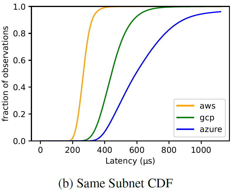
Many, if not all, practical distributed systems rely on partial synchrony in one way or another, be it a failure detection, a lease mechanism, or some optimization that takes advantage of synchrony to avoid doing a bunch of extra work. These partial synchrony approaches need to know some crucial parameters about their world to estimate…
-
Metastable Failures in the Wild
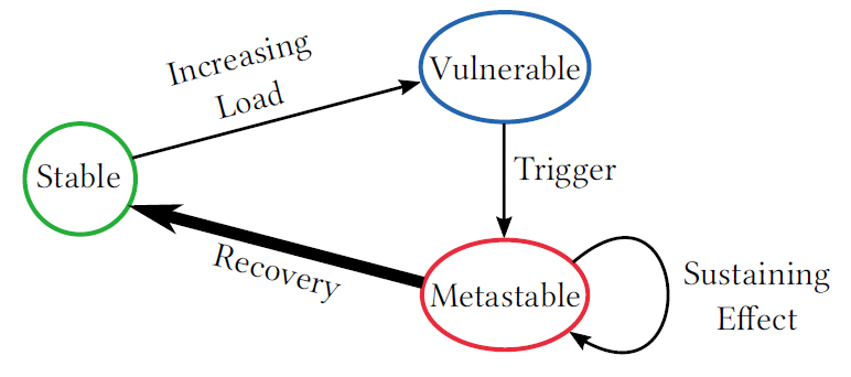
Metastable failures in distributed systems are failures that “feed” and strengthen their own “failed” condition. The main characteristic of a metastable failure is a positive feedback loop that keeps the system in a degraded/failed state. These failures are hard to spot, as they always start with some other distraction — some trigger event that nudges…
-
How to Read Computer Science (Systems) Papers using Shampoo Algorithm
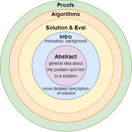
I think most academics had to answer a question on how to approach papers. It is the beginning of the semester and a new academic year, and I have heard this question quite a lot in the past two weeks. Interestingly enough, I believe that almost every academic active on the Internet has written about…
-
Scalable but Wasteful or Why Fast Replication Protocols are Actually Slow
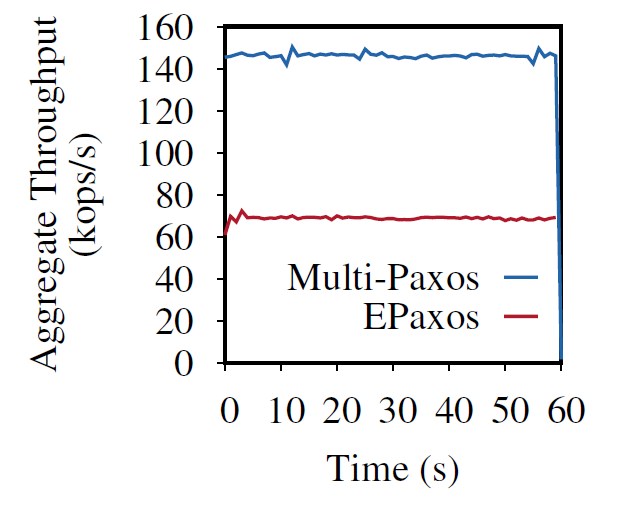
In the last decade or so, quite a few new state machine replication protocols emerged in the literature and the internet. I am “guilty” of this myself, with the PigPaxos appearing in this year’s SIGMOD and the PQR paper at HotStorage’19. There are better-known examples as well — EPaxos inspired a lot of development in…
-
Metastable Failures in Distributed Systems
Metastability is a stable state of a dynamical system other than the system’s state of least energy. – Wikipedia Distributed systems often fail spectacularly and unpredictably. They are a cause for a headache and sleepless on-call nights for way too many engineers. And this is despite lots of efforts to understand the failures, and all…
-
Looking at State and Operational Consistency
Recently I rediscovered the “The many faces of consistency” paper by Marcos Aguilera and Doug Terry. When I first read the paper two years ago, I largely dismissed it as trivial, and, oh boy, now I realized how wrong I was at that time. It is easy to read for sure, and may appear as…
-
Python, Numpy and a Programmer Error: Story of a Bizarre Bug
While recently working on my performance analysis for Paxos-style protocols, I uncovered some weird quirks about python and numpy. Ultimately, the problem was with my code, however the symptoms of the issue looked extremely bizarre at first. Modeling WPaxos required doing a series of computations with numpy. In each step, I used numpy to do…
-
Retroscoping Zookeeper Staleness
ZooKeeper is a popular coordination service used as part of many large scale distributed systems. ZooKeeper provides a file-system inspired abstraction to the users on top of its replicated key-value store. Like other Paxos-inspired protocols, ZooKeeper is typically deployed on at least 3 nodes, and can tolerate F node failure for a cluster of size…
-
Why Government IT is Expensive and Archaic
Disclaimer: I do not work for the government, and my rant below is based on my very limited exposure to how IT works at the US government setting. Why Government IT is Expensive and Archaic? I think, this can be a very long discussion, but I do have a quick answer: standards imposed by government…
-
New Blog
My name is Aleksey Charapko, I am a computer science student at the University at Buffalo. In this blog I will try to write on mostly technical topics that I am interested in.
Search
Recent Posts
- Paper #196. The Sunk Carbon Fallacy: Rethinking Carbon Footprint Metrics for Effective Carbon-Aware Scheduling
- Paper #193. Databases in the Era of Memory-Centric Computing
- Paper #192. OLTP Through the Looking Glass 16 Years Later: Communication is the New Bottleneck
- Paper #191: Occam’s Razor for Distributed Protocols
- Spring 2025 Reading List (Papers ##191-200)
Categories
- One Page Summary (10)
- Other Thoughts (10)
- Paper Review and Summary (14)
- Pile of Eternal Rejections (2)
- Playing Around (14)
- Reading Group (103)
- RG Special Session (4)
- Teaching (2)