My last metastable blog post discussed the interactions between systems and components and how they can lead to metastable failures. Specifically, I looked at interactions between systems/components and how signals can be misinterpreted by different systems due to ambiguity — a timeout may mean a transient fault that can be fixed by retrying, but it may also mean a catastrophic overload where retrying only makes things worse. This leads to an important realization: some common action systems take in response to signals can be good under some assumptions and bad under others.
Last month, Todd Porter from Meta, Dave Maier from Portland State, and I gave a talk at SREConn Americas on Metastability in Recovery. This talk discusses how cross-system interactions and ambiguous assumptions can make recovery of system of systems impossible due to cascading amplifications and feedback loops.
It is a common fact that failures can spread. A lot of engineering effort is often put into siloing/compartmentalizing systems to reduce the blast radius. But if failures can spread, so do the recoveries from failures. Failures (often) spread visibly — as one system starts to affect another, alarms begin to sound on the newly affected system. The recoveries spread differently and often more silently. Even if we successfully isolate failures and prevent them from propagating directly to other components, it does not mean that recoveries from these failures will not spread. Consider two systems: A and B; system A experiences a problem, but the problem remains isolated to A. However, system B usually receives its work from A, and while A is failing, it sends less work to B. The recovery of A, however, can be rather unexpected to B — it now starts receiving all the work, and maybe more, as A’s recovery tries to process and ship the backlog to B.
These recovery interactions formed a cascade in which the recovery of one system, system A, which we can call a “dependee,” for lack of a better term, triggers the recovery of its dependent, system B. In some cases, the dependent’s recovery may require more resources than doing the same amount of work in the common, non-recovery case. As a result, we build an amplified cascade, and it, like an avalanche picking up more snow as it moves down slope, requires more and more work to complete for recovery of the whole system.
This alone is a problem. Not a metastable one, but still a big one that can snowball into the inability to recover the system. However, unlike an avalanche, system recovery can also have feedback mechanisms that create extra work for systems that have already recovered upstream. And such feedback, creating extra work upstream, can create a perpetual loop of failures and recoveries.
The Example
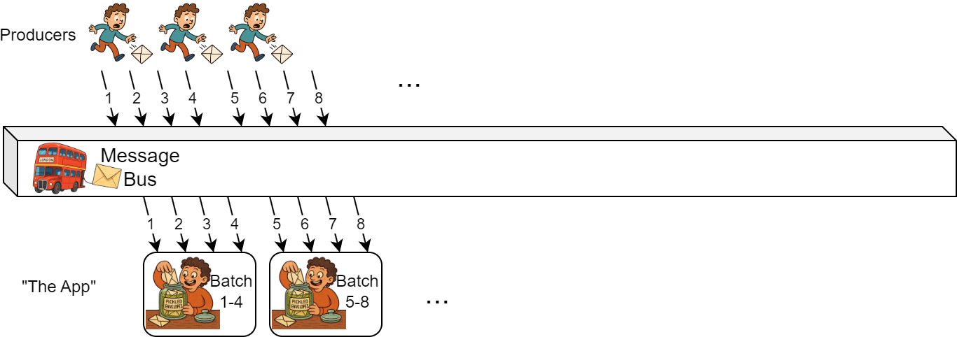
Let’s consider an example. Imagine a typical producer-consumer system: producers write some data to a shared message bus (think Apache Kafka), and producers fetch the data and perform some expensive computation before shipping the result downstream to other services/components. In our case, the system produces time-series data, and consumers fetch this data for an entire time slice (e.g., an hour’s worth of a specific data stream) before performing an “expensive computation”. I illustrate this simple app with the image below:
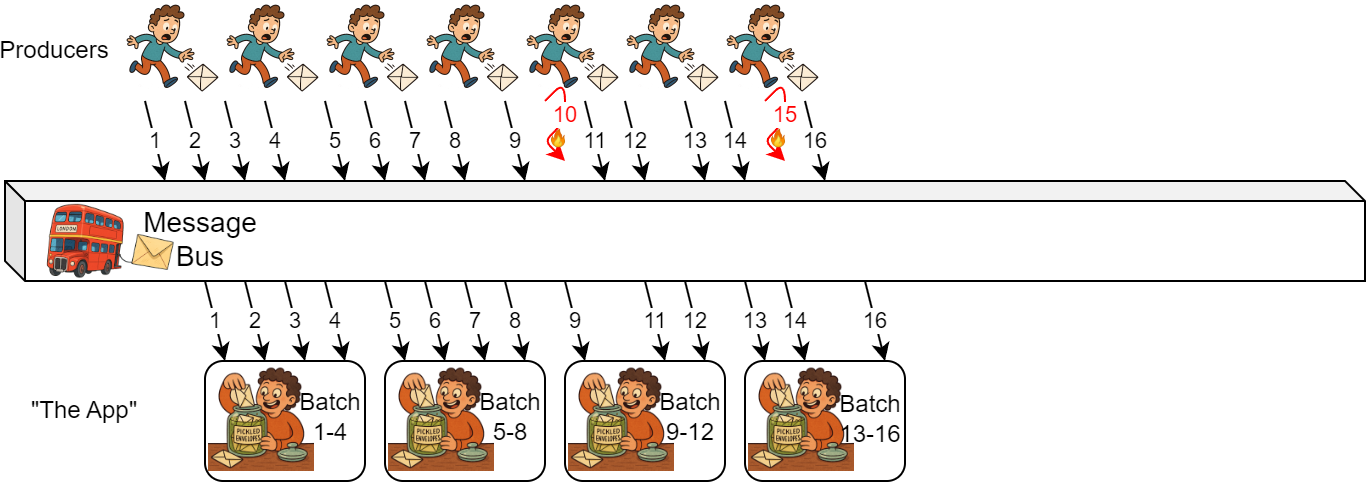
However, something has happened on the producer side that caused some data to be missing and not arrive at the message bus on time (items 10 and 15 in the image below). The consumer side is unaware that some data is missing, so it follows its regular logic: it waits for all data in a specific time range to stop arriving, and then batches it and performs the “expensive computation.”
But what happens when the producer recovers, and the missing data finally arrives at the message bus and is delivered to the consumer? From the producer’s perspective, delivering missing data may not have cost that much more — the same amount of work done a bit later. From the message bus’s perspective, it is the same. But for our consumer, it is a problem.
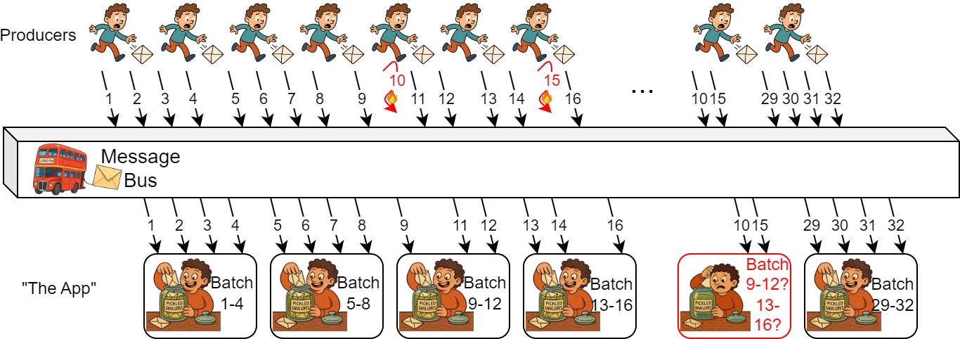
The consumer app, despite never failing, is being asked to perform a recovery action after receiving belated data. The late data belongs to batches done a long time ago, so the consumer app needs to recompute them. This re-computation of a batch is expensive. Way more expensive than including the missed data in the original batch computation, had it received the data on time. This consumer cost, however, is just a part of the problem. The app also does not keep old data after it finishes the “very expensive computation,” and now needs to refetch the old data it has already received once. This is the feedback upstream into the message bus; refetching the data places additional load on it.
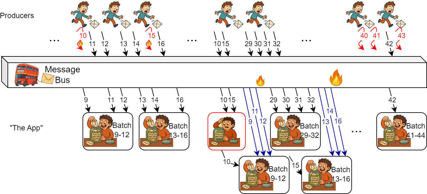
This additional load due to feedback can start a loop. If the additional load is high, the message bus will slow down and may not accept new data quickly enough, or it may fail to send data to consumers on time due to overload and queuing. This will create more batches that will need to recover on the consumer side, and as we remember, this recovery creates the upstream feedback into the message bus, making it run even slower.
The Formalism
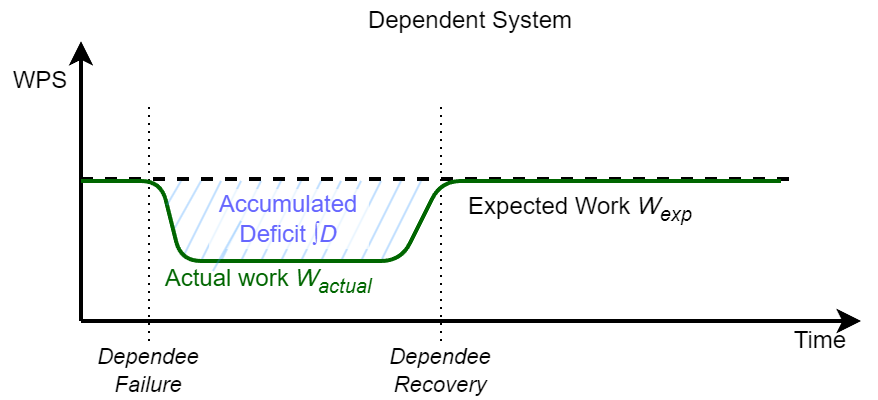
As I mentioned, the recoveries cascade and cause ripples of recoveries even in the systems that may not have actually failed, systems that simply did not do all the usual work because the upstream failure did not provide that work. So if we have a dependee failure, it creates a deficit of work sent to the dependent systems. This deficit or backlog accumulates over time. When the dependee recovers, the deficit must also be recovered by the dependee and the dependent.
We have three broad recovery modes:
- No recovery: the deficit/backlog is ignored. This is good for metastability, as it stops the recovery cascade.
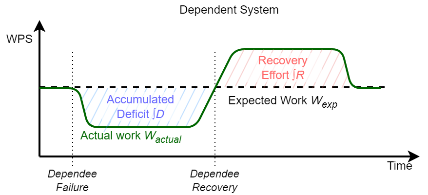
- Additive recovery: the deficit recovery requires the same work (or less!) as it would have taken to do this work without recovery. Think of this as a time-displacement for the work done. Instead of doing it at the expected time, we do this work later. This additional work sits on top of the usual work still to be done, so additive recovery, due to the time displacement, requires more resources on the dependent system.
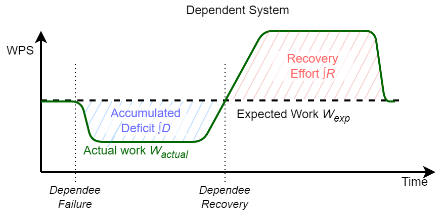
Amplified Recovery: This is the bad case. The recovery of a unit of deficit takes more resources than doing that unit of work in a common case. Not only is the work time-displaced and requires more resources from the dependent, but it may also require substantially more resources. Amplified recovery also introduces the possibility of feedback to the dependee/upstream system, which can lead to metastable failures (as I’ve seen in my simulations, the feedback loop may also develop within the dependent system itself rather than upstream, in which case even additive recovery is vulnerable to metastable failures).
The “Mismatches”
If we look at the causes of amplification, they are numerous. We identify a few common cases of mismatches — situations where the system’s expectations do not match the realities of the environment.
Thermal Mismatch: This occurs when recovery, due to its time-displacement, no longer benefits from the faster warm data path. For instance, in our example app, refetching that data from the message bus may hit “cold storage” rather than the “hot” cache, since the data was not used for a while.
Granularity Mismatch: the unit of recovery in the dependent system does not match the unit of deficit or backlog, so even a small backlog may require significant recovery effort. In our example, a missing data item, which may constitute a fraction of a percent of all data in a batch, can cause the entire batch’s worth of data to be refetched and the whole batch recomputed — a very high price to pay for recovering something small.
Cost Mismatch: as systems process work, it can take different execution paths. These paths may result in different execution costs (resource-wise). If the recovery is running though an inherently slower paths, it will create the amplification.
General Expectation Mismatch: This one is kind of a catch-all for a lot of things. But it is common to assume and expect certain behaviors, only to find that they do not hold in rare or extreme cases. Recovery paths tend to be less exercised, so they are rarer cases and are more likely to violate expectations and assumptions.
The Actions
There are a few things we can do about the cascading recovery, though.
Prefer Additive Recovery. First of all, if we need to clean the backlog in case of recoveries, we really should design the system to stay in the Additive Recovery mode. This means avoiding granularity mismatches and designing for additive, incremental recovery rather than the expensive recomputation of larger work units.
Budget Recovery and Stream Shaping. Avoid doing all the deficits at once. Doing more work quickly leads to using more resources quickly. Spreading backlog recovery over longer periods or streams on a capped “recovery budget” can help avoid large load spikes in the dependent system.
Scale Up for Recovery. The cascading recovery is somewhat anticipated. When the dependee recovers, it will send the backlog downstream. Increasing dependents’ capacity in advance can help handle a burst of work. This works best for Additive Recovery, where the cost of doing recovery work is known.
Adequate end-to-end Resource Provisioning. Make sure resources match recovery requirements, especially end-to-end! It is important to understand the amplifications happening and provide adequate resources. Scaling up (previous point) can help, but only when taken holistically. If we make one component stronger or more capable without making its dependents also able to handle more work, we are setting up for a different failure.
Avoid the Cold Path and Prewarm for Recovery. The time-displacement of recovery means that the recovery work may not be done at the best time. In our example, the time factor means consumers no longer have the batch data; refetching it from the message bus amplifies the cost, but because this refetch happens later, the message bus may have moved the data from in-memory cache to storage, further increasing the cost. Prewarming cold data in systems may help avoid some amplification costs.
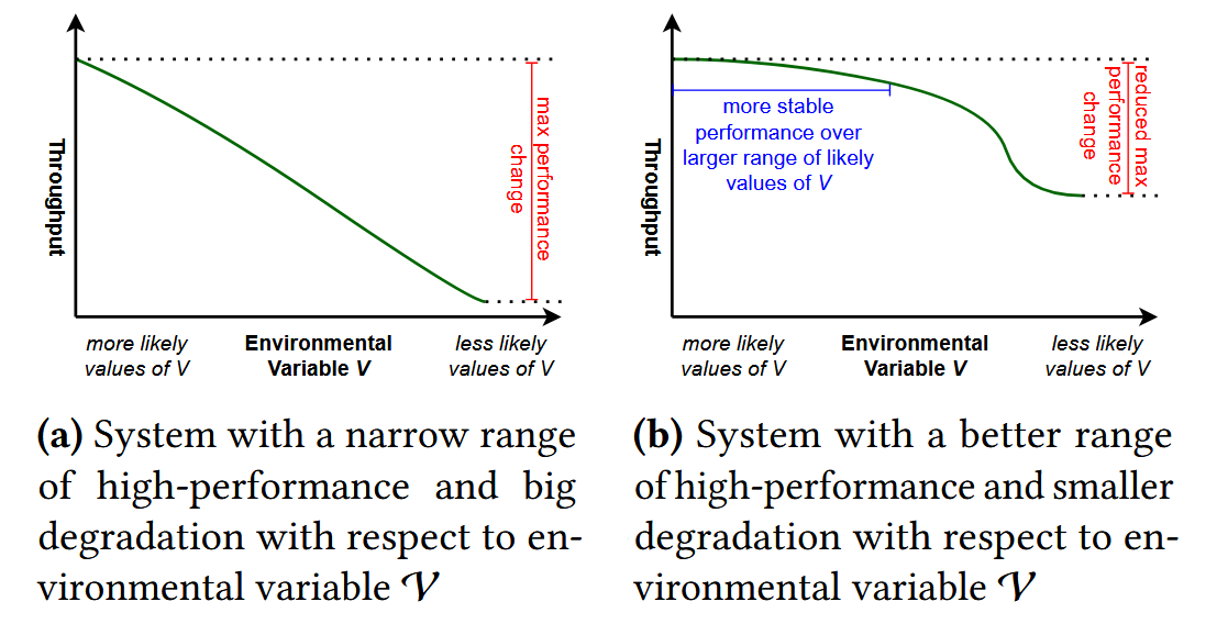
Design for Recovery Path. The happy path through the systems is only happy until a failure occurs. Designing systems for recoverability may mean a less-optimized common case, but a better “performance gradient” — the difference between the capacity/performance of a system in a common vs. exceptional case. In our example, designing for a recovery path would not only include additive recovery but also minimize other types of mismatches, such as cost mismatch or thermal mismatch.
The Simulation
To better understand how the problem develops, I simulated the above example in MESSI, my still-in-development-but-already-useful performance simulation tool designed to study metastable behaviors. A system in MESSI is represented as a graph of Logic Nodes and Processors, where Logic Nodes have necessary algorithms and protocols and provide work routing, while Processors simulate all temporal behaviors, such as service times and queuing. The simulator operates in discrete time and sends work items through the system to simulate requests and their progression through the components.
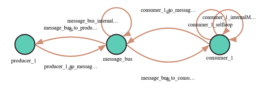
Our simulated system consists of just three Logic Nodes: one to encode the producers, another for simple message-bus logic, and the third for the consumer app. The nodes are connected via a simulated network. Also note that some nodes have edges that start and end at the same node; these self-loop edges often represent delays/processing for a particular component. All these result in the system graph shown here.
The producers create a ProduceRequestResponse request to send small time-series data items to the message bus. I simplified the system a bit and made the consumer initiate the data transfer from the message bus. The consumer periodically creates a ConsumerRequestResponse request to the message bus to fetch available data. In response to this request, the message bus sends the accumulated messages that were not sent before. The consumer’s ConsumerRequestResponse may also specify a time range, in which case the message bus will resend the messages within that range. Finally, the consumer also creates BatchProcessingQItem requests that are not sent to any other node; instead, they are used to drive the simulation of performing the “expensive computation” on the batch of data.
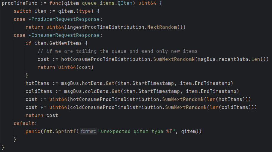
In this simulation, I used a multi-worker queue abstraction to simulate processing delays at both the message bus and the consumer app components. The processing delays at the message bus depend on the type of work (ingest or send), the number of simulated data items being sent, and their cold/hot status (with cold items requiring more resources to fetch from storage before they can be sent). I do not simulate actual storage/IO costs or processing interruptions due to disk IO in this model (but I have done so for other models/problems). Similarly, the consumer app simulates the cost of receiving data from the message bus and the cost of performing “expensive computation” proportional to the amount of data received. The snippet here shows a function that defines the simulated cost of doing work on the message bus by drawing from and aggregating costs from several distributions.
What Does Simulation Tell Us?
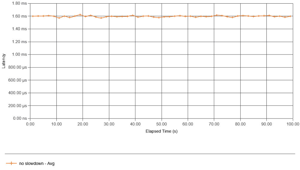
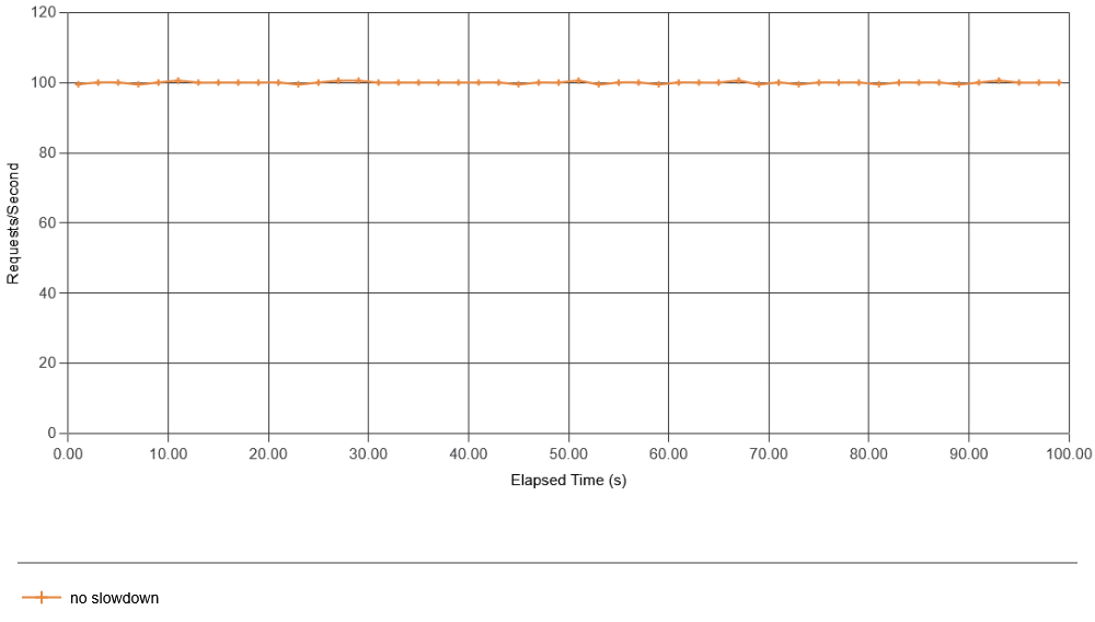
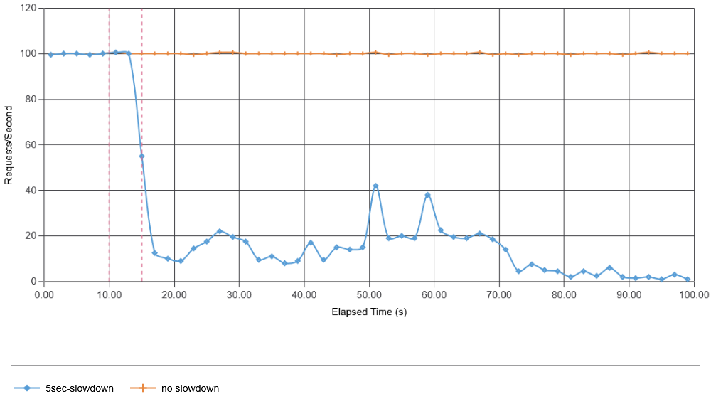
First, I simulate the standard case — the behavior of a system in a steady state without data production failures. As a metric, I look at consumer apps’ interactions with the message bus (both latency and requests per second). Other metrics work too and may give additional insight. For instance, the latency and throughput of data production may better show message bus overload, while the latency of batch creation may better show consumer app overload. Anyway, for brevity, I focus on just the consumer app’s interaction with the message bus. The consumer was configured to request new data from the message bus every 10 ms, so we expect about 100 interactions per second. The figure below shows just that, as the system operates without any failures introduced on the producer side.
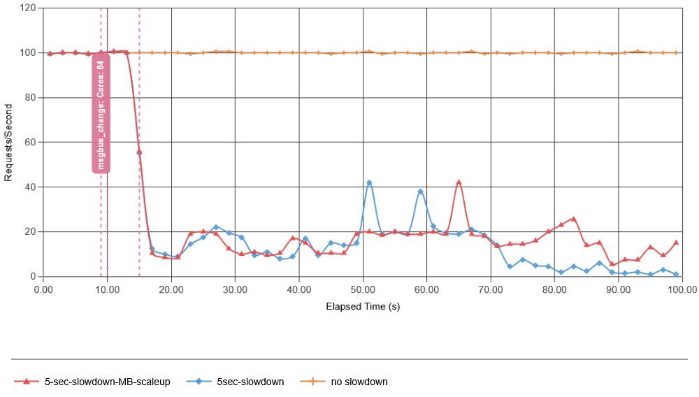
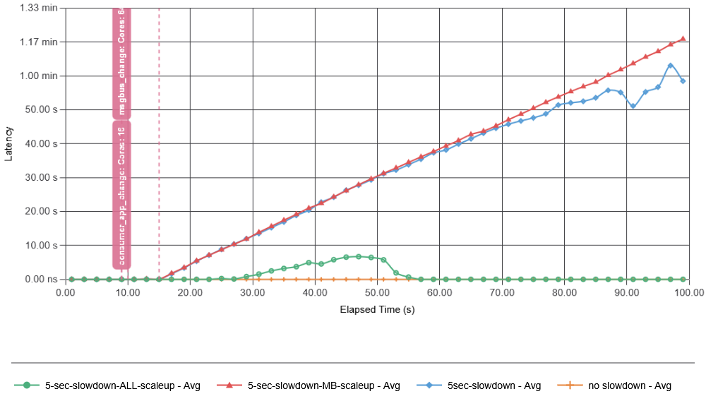
Next, I introduced a 5-second-long failure at the 10-second mark. This failure delays just 1% of the produced data, causing it to arrive later. In this case (and all other simulations shown here), I had the app construct the batches of 1-second in duration, so if the 1% of data arrives longer than some configured wait threshold (500 ms of no additional data for a batch “seals” it for processing), the batch will be made without the missing data. It turns out that this 1% of missing data was enough to cause a catastrophic metastable failure. The pink vertical lines indicate the start and stop of the 1% failure. Here, we clearly see that the consumer app is no longer able to ask/retrieve data from the message bus, with average data retrieval latency exceeding 500 ms, far exceeding the 500 ms batch sealing time. This creates many more incomplete batches that will need to be recovered when they start receiving belated data.
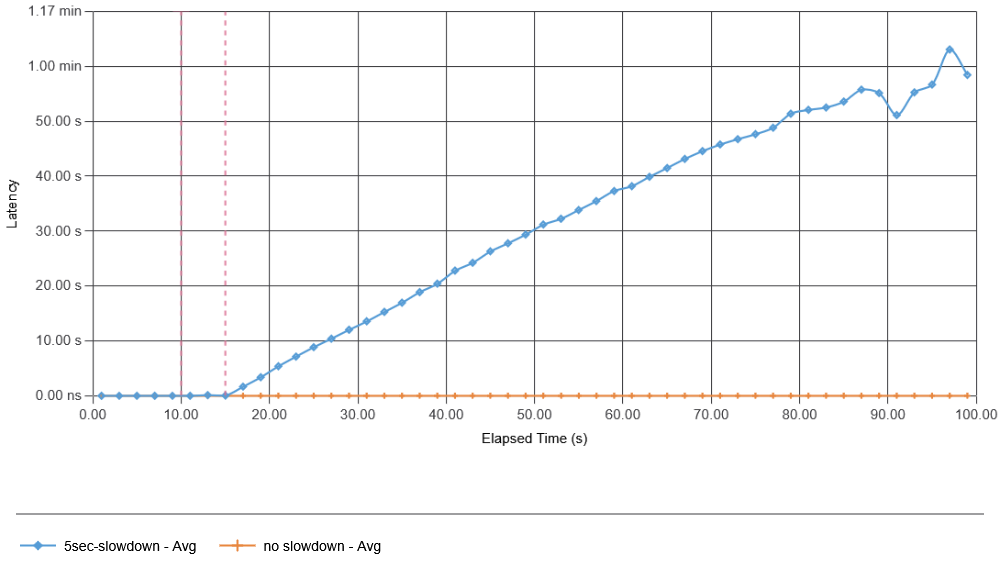
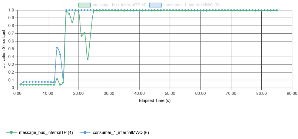
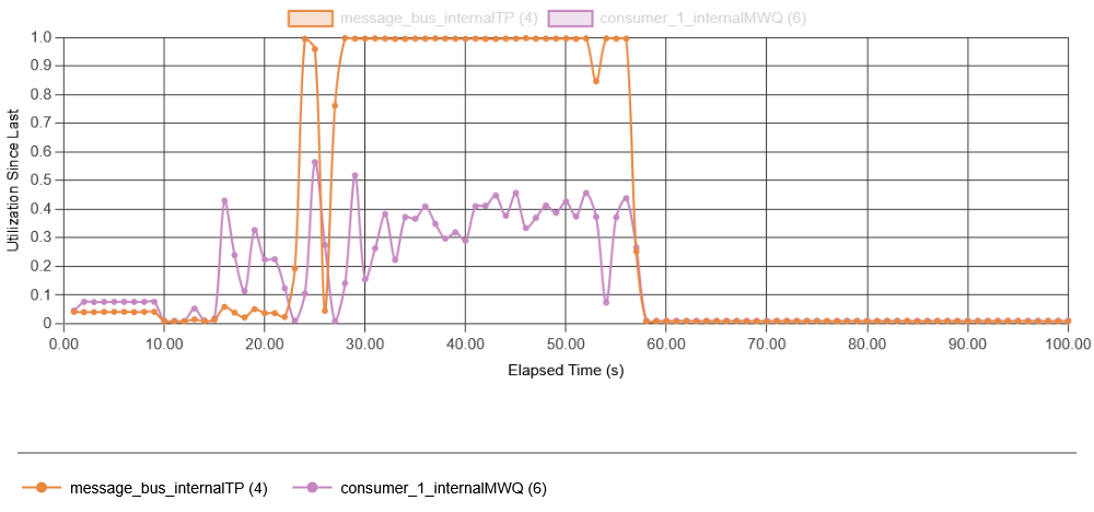
These results show how quickly a failure can develop in our example system, even with a small initial failure rate of 1% missing data. In fact, the simulation shows that we quickly corrupt more batches with delayed data due to overload of the message bus than the initial failure did. While the time scale of this test app may not match that of the real app Todd talked about at SREConn, it captures a very similar behavior to that observed in a real system. The cause of the high latency in data fetching is the overload of system components. Recall that failure starts at 10 seconds, so by 11.5 seconds, the first batch with missing data may be completed by the consumer, and in another second or so, that batch may undergo repair. In fact, in this simulation, one batch may undergo multiple repairs, making the feedback much stronger, as even more delayed data may arrive after the first repair. All of this results in a very quick resource exhaustion on both the message bus and the consumer app (note that both initially work with under 10% utilization):
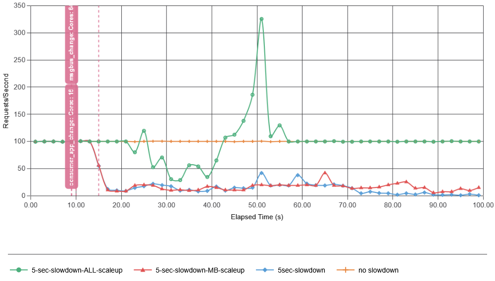
I tried adding some resources in anticipation of recovery and made message bus nearly 20 times faster. That did not help at all!
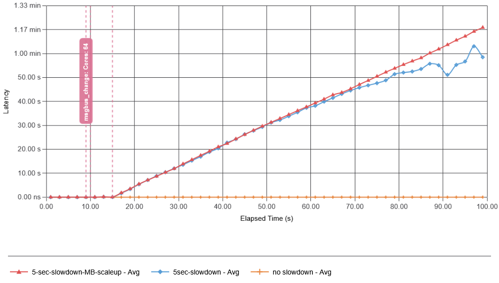
The reason for adding resources to the message bus was that it is the message bus that gets overloaded by the feedback. But that did not help, since even if the message bus has resources to continue ingesting data and serving data to the app, the app itself, overloaded by the recovery amplification, cannot accept data in time, still leaving us with the problem of creating more incomplete batches that will undergo recovery later as more data arrives. In fact, it required scaling up both the message bus and the app to avoid a metastable failure. And the interesting thing was that… it was not as critical to briefly overload the message bus as it was to overload the consumer app. In fact, this broke my initial assumption that the message bus is the primary driver of the failure. Instead, consumer overload may be largely responsible for the feedback loop, as an overloaded consumer cannot ingest data from the message bus quickly enough, causing broken batches.
Simulating the problem was a fun exercise. I covered only some of the data gleaned from it, but running the simulation increased my understanding of the problem, the loops, and their impacts on the whole system. The simulation also allows playing with many hypothetical scenarios and trying many solutions without the risk/cost/effort of a real system. And finally, simulations will also be helpful in our new “agentic” world, as they can provide quick feedback to agents to refine and test algorithms, designs, and architectures.