In the past few months our lab has been doing a lot of work with different flavors of paxos consensus algorithm. Paxos and its numerous flavors are widely used in today’s cloud infrastructure. Distributed systems rely on it for many different tasks to ensure safe operation. For instance, coordination services use some consensus protocol flavor to provide services like leader election, cluster membership, service discovery and metadata management. Databases, such as Spanner or CockroachDB, use paxos to provide fault tolerant-replication of data across nodes or even datacenters.
If you work with Paxos, or had to deal with it at some point, you probably heard that it does not scale well to large number of nodes. ”Five nodes is ideal, do not try more” rhetoric has been repeated many times by many people and it gets engraved into one’s mind. ZooKeeper’s Administrator’s guide mentions 3 and 5 server deployments. Fairly recent epaxos provides evaluation on 3 and 5 node deployments in their paper. Paxos Made Live paper also mentions five nodes as typical Chubby deployment.
But why five servers is such a magical number in the Paxos world? The most common answer is along the lines of ”Increasing the number of servers increases the quorum size, making the paxos round leader wait for more messages to come to reach consensus”. This explanation is straightforward on the surface, after all, waiting for n nodes to reply should take longer than waiting for n − 1. The question then becomes why waiting for more replies is expensive? I thought the answer would be largely network related, but it appears to be more complex.
Modeling Paxos Performance: First Attempt
To answer this, I tried to model the non-faulty paxos execution time by looking at message exchange between nodes in the cluster. In the nutshell, running a phase of paxos requires one round-trip-time (RTT) between a node and its peers: the node broadcasts the message and waits for the quorum to reply. With network arguably being the slowest part, I can try to express the paxos phase performance through the communication delays
First, let me define some variables to model a phase of paxos:
- \(r_l\) – message RTT in local area network
- \(\mu_l\) – average message RTT in local area network
- \(\sigma_l\) – standard deviation of message RTT in local area network
- \(N\) – number of nodes participating in a paxos phase
- \(q\) – quorum size. For a majority quorum \(q=\left \lfloor{\frac{N}{2}}\right \rfloor +1\)
- \(m_s\) – time to serialize a message
- \(m_d\) – time to deserialize and process a message. This involves various message-related round tasks, such as ballot comparisons, log maintenance/updated, etc.
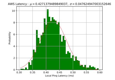
I assume that the network performance, at least in the local area, is normally distributed. Figure 1 shows a normalized histogram (shaded area is equal to 1) of latencies of approximately 2,000 ping requests within an AWS region.
RTT \(r_l\) for every message is drawn from a normal distribution \(\mathcal{N}(\mu_l+m_s+m_d, \sigma_l^2)\). This distribution simulates RTTs with additional static, non-variable delay for serialization and deserialization. As such, the only variability so far is due to the network behavior.
In order to run a round of paxos, a node needs to send \(N − 1\) messages. That is, a node sends a message to every other node except for itself. I assume a ”leader” is also an acceptor with a short-circuit behavior, where a it does not need to send a vote to itself over a network.
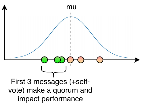
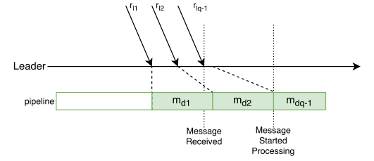
Out of the \(N − 1\) messages sent, only \(q − 1\) messages actually matter. Upon receiving \(q − 1\) successful (once again, assuming non-faulty execution) replies a node has achieved a quorum and can finish the round (Figure 2). We can simulate this by drawing \(N −1\) random RTTs \(r_{l1}, r_{l2},…, r_{lN-1}\) from \(\mathcal{N}(\mu_l+m_s+m_d, \sigma_l^2)\) and sorting them. The \(q − 1\) fastest message \(r_{lq−1} \) is the one carrying the last vote to make up a quorum, thus after processing this message, the node no longer needs to wait for other messages to come.
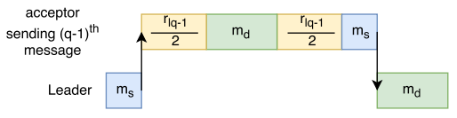
Assuming that a node broadcasts all messages at the same time, message RTT \(r_{lq−1} \) can then be used to express the latency \(L_r\) for the entire round: \(L_r = m_s + r_{lq−1} + m_d\). Figure 3 visually represents the paxos round expressed in the formula.
Does the Model Make Sense?
With this simple model, I can simulate paxos execution. In multi-paxos optimization where phase-1 is used to primarily pick a stable leader and phase-2 repeats a number of times, the performance of paxos is approximated by just looking at phase-2. If \(m_s\) and \(m_d\) are constant, the variability in performance is only due to the network fluctuations.
I created a small python script to run such simulation, as if a single client was interacting with the paxos synchronously one command at a time. Figure 4 illustrates the results with \(m_s = m_d = 0.01 ms\) and network parameters taken from AWS ping latency figure.
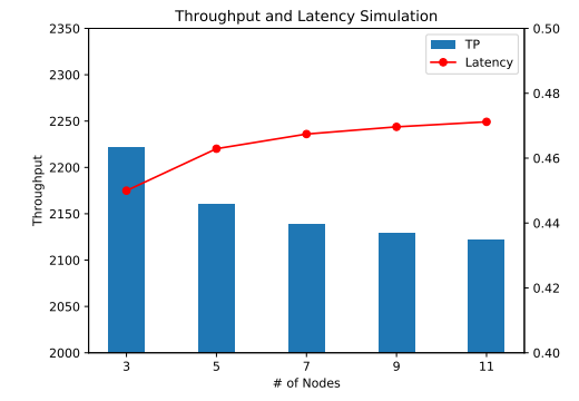
At the first glance, we observe degradation in throughput and increase in latency. However, the performance decreases very slowly, and once I reach 9 nodes, the performance stays almost flat. This is very different from the data we have observed on our actual paxos implementation. Figure 5 shows the throughput and latency from a few concurrent clients interacting with the protocol.
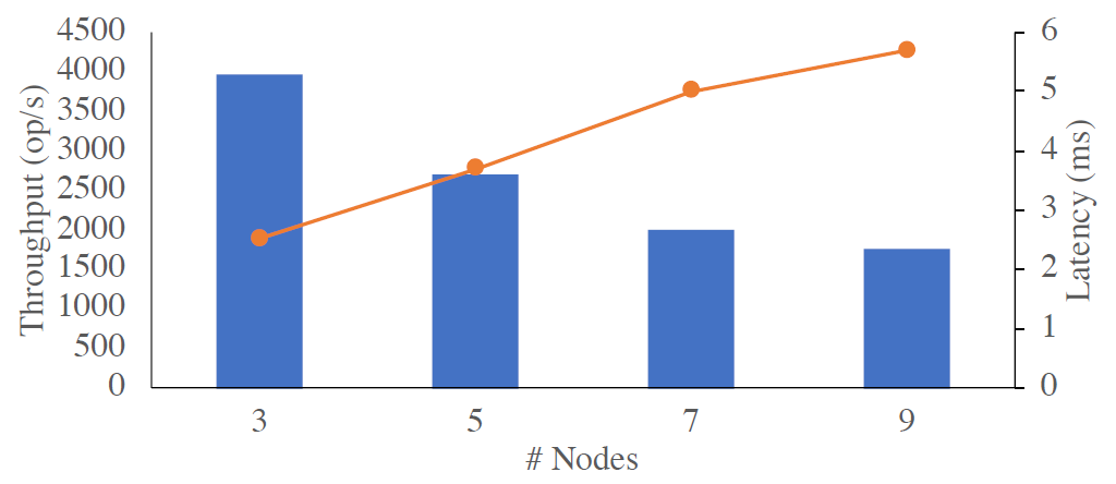
The first thing that catches my attention is the performance degradation between the 3 and 5 node deployments. On the simulation, the difference in throughput was only 2.8%, while real paxos degraded by astonishing 30%. As the cluster size increases, beyond 5 nodes, the real paxos also appear to degrade quicker.
Clearly, the network variability alone cannot explain the performance hit from increasing the number of nodes. So what is missing from the simple model that greatly impacts the performance as the cluster grows?
Towards an Improved Model
Starting from the obvious, the per-message serialization \(m_s\) and processing \(m_d\) overheads are not static constant parameters, instead they introduce some variance as well. However, \(m_s\) and \(m_d\) are small to start with, and making them introduce additional variance to the model will make it better, but it will not change the overall model simulation much.
Assuming that \(m_s\) is drawn from a normal distribution \(\mathcal{N}(\mu_{ms}, \sigma_{ms}^2)\) and \(m_d\) is similarly drawn from \(\mathcal{N}(\mu_{md}, \sigma_{md}^2)\), then the message RTT time \(r_{l}\) must be drawn from \(\mathcal{N}(\mu_l+\mu_{ms}+\mu_{md}, \sigma_l^2 + \sigma_{ms}^2 + \sigma_{md}^2)\). Making this changes to the model resulted in a difference between 3 and 5 node simulations to grow from 2.8% to 2.9% with \(\mu_{ms} = \mu_{md} = 0.01\) and \(\sigma_{ms} = \sigma_{md} = 0.002\) (some arbitrary values that make little impact, unless same magnitude as network mean and standard deviation).
Introducing the variability to message overheads \(m_s\) and \(m_d\) still does not account for these overheads being dependent on the number of node in the cluster. The dependence on \(N\) is not direct, and instead the per-message costs increase as the number of messages that a server needs to handle grows. This puts a ”leader” node repeating the phase-2 of paxos in a more vulnerable position as it will experience the increased traffic.
To understand how message serialization and processing depends on the number of messages exchanged, we need to consider the implementation of application’s network layers. Often times, as an application receives the message, it will use one or more processing queues or pipelines to deserialize the message and dispatch it to the appropriate handler for processing.
Let’s consider an example with just one such pipeline. If the queue is empty upon message arrival, it will get to deserialize with no further delay. However, when there are other messages in the queue, the new message has to wait for it turn to be processed.
A single Paxos round has a bursty network utilization, especially at the leader. This is because the leader node first broadcasts a messages and then receives multiple replies at roughly the same time. If the message deserialization has not finished before the next message arrives, then the pipeline gets clogged. Further messages potentially make the issue worse by growing the queue, as shown in Figure \ref{fig:pipeline_clogged}.
Obviously, having multiple parallel pipelines can help, given that they are balanced and there are enough compute resources to run them. However, the problem can also get worse when we start running rounds concurrently (i.e. multiple clients interact with paxos). In such scenario, messages from different rounds will compete for the fixed number of processing queues.
Where does this leave me with trying to model paxos round performance? I need to account for a number of additional factors, such as the number of message-processing queues/pipelines/threads, the rate of message deserialization at each queue, and the number of concurrent paxos rounds. Oh, and since the messages arriving after the quorum has been reached still need to get deserialized, they will contribute to how clogged the pipelines are.
I will pick up from this point onwards in some future post. I will also try to look at flexible quorums and our WPaxos protocol.
Update (3/10/2018):